Computer Science Department, Colorado School of Mines
What is an Image and how is it formed?
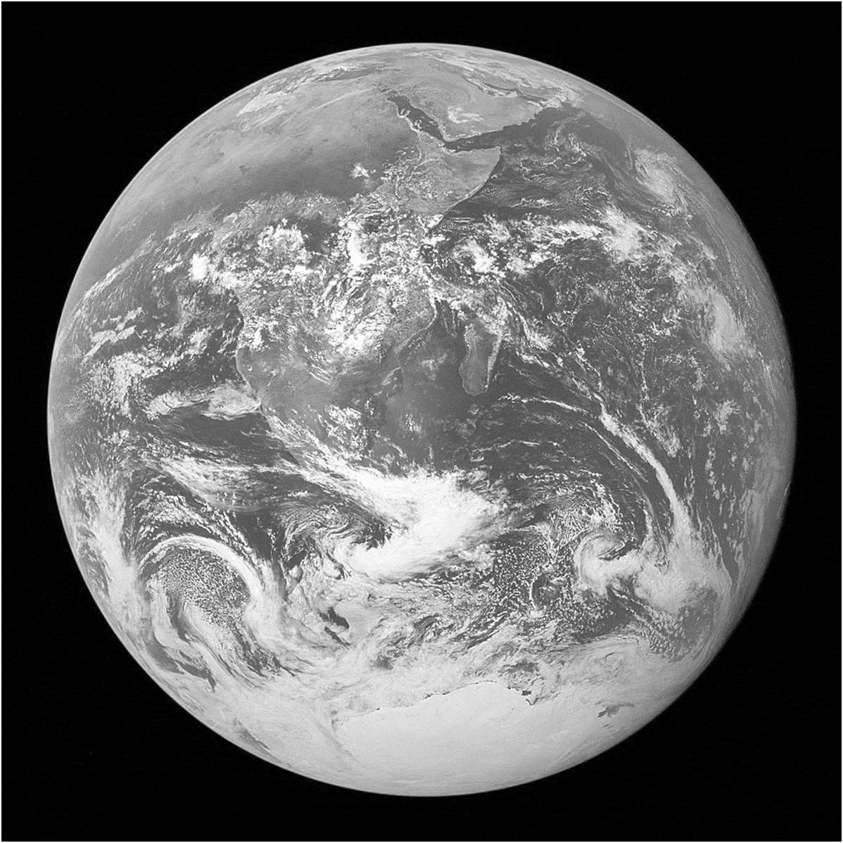
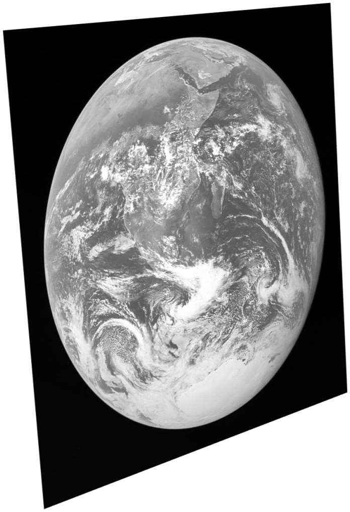
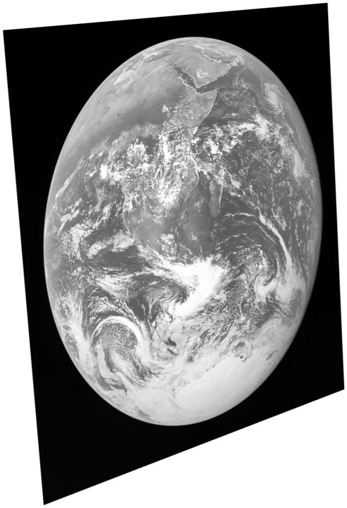
Blue Marble, NASA / Apollo 17
Image Formation
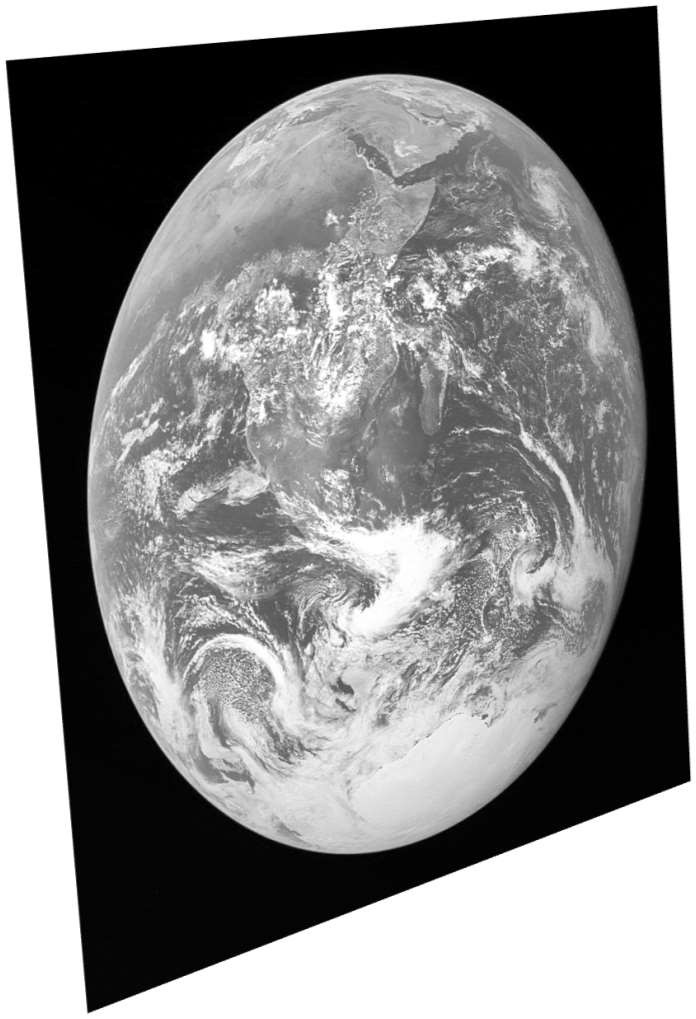
Scene / object
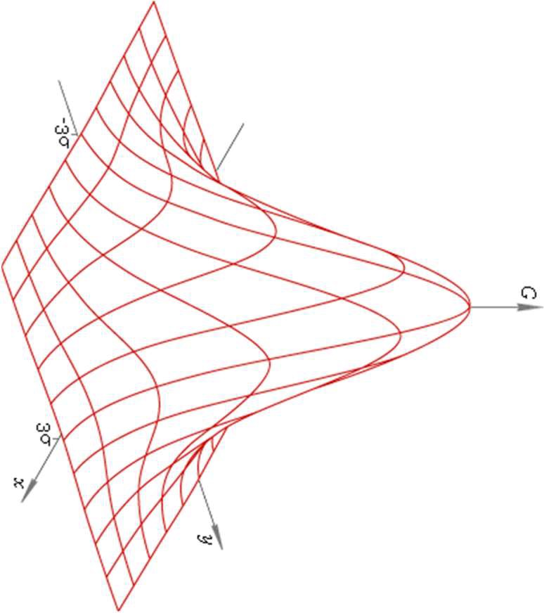
Light as a signal
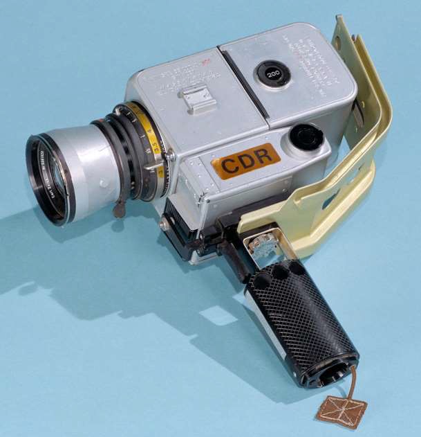
Camera / sensor
A camera measures light from the world and turns it into a digital image.
Signal
Signal: A (multi-dimensional) function that contains information about a phenomenon (e.g., light, heat, gravity, sound, pressure, motion).
Signals can be continuous, such as light in the physical world.
Measurements are often discrete samples of that continuous signal.
Sampling reduces a continuous signal to a finite set of values.
Sampling in 1D
Sampling a 1D continuous function returns a vector whose elements are values of that function at selected sample points.
Instead of the full function, we store values at selected locations.
Sampling in 2D
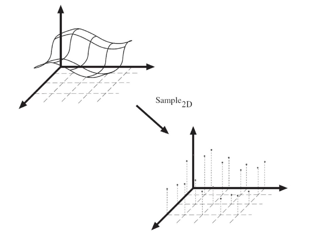
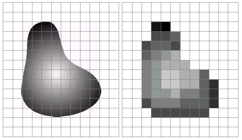
Sampling a 2D function returns a matrix.
2D Image
Image: A sampling of a function that contains information about a 2D signal.
The function stores brightness or intensity.
The image samples brightness along the \(x\) and \(y\) dimensions.
A video can be viewed as a time-varying 2D image signal: \((x, y, t)\).
Note
Cameras observe a 2D projection of the 3D world.
Examples of 2D Images
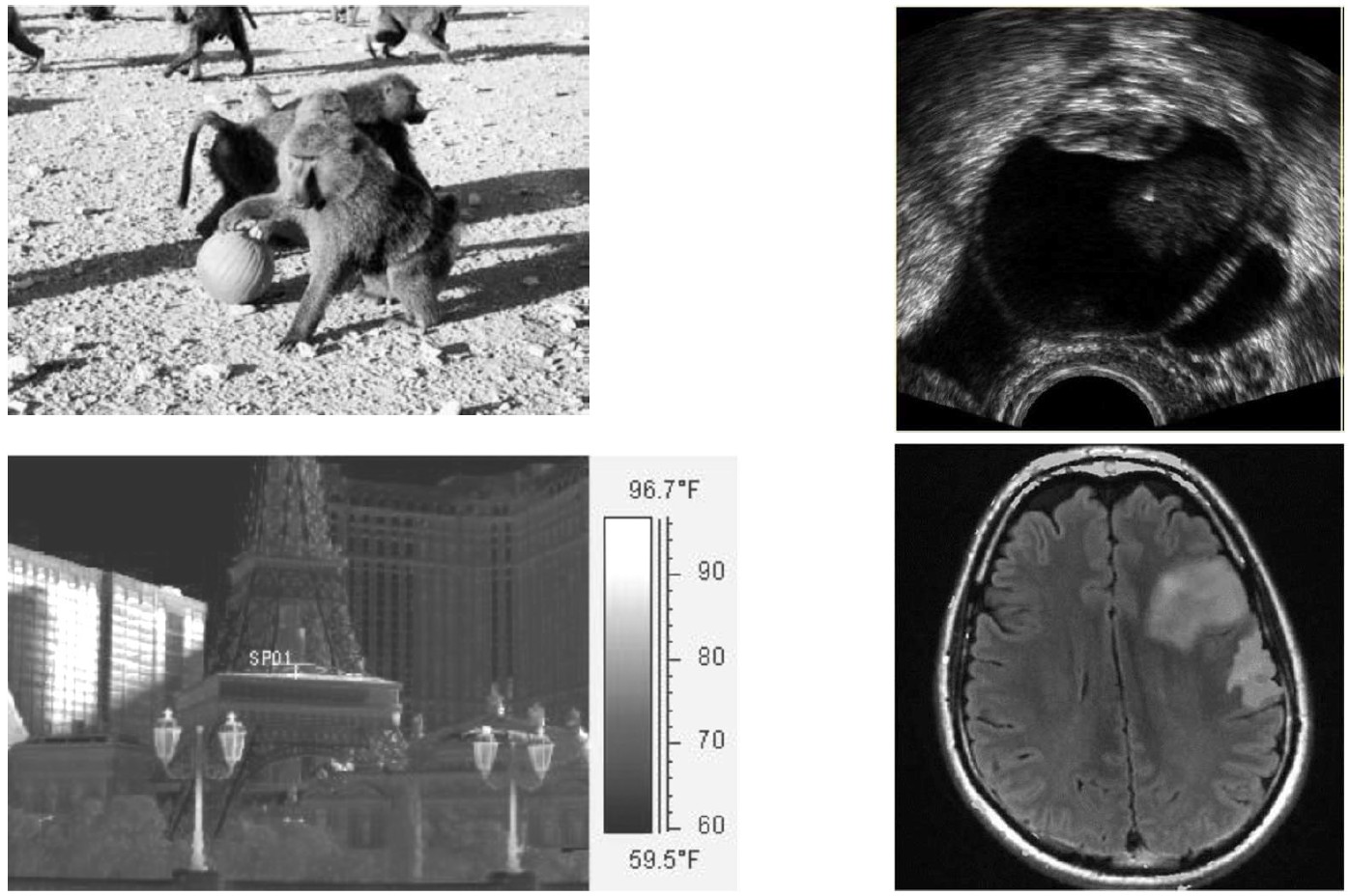
2D images appear in many sensing modalities:
Natural images
Thermal images
Satellite/aerial images
Microscopy
Ultrasound
MRI / CT slices
Radar images
Depth images
Note
The signal may not always be visible light. An image arranges what we have measured over a 2D domain.
Sampling in Practice
World / scene
Continuous signal
Camera
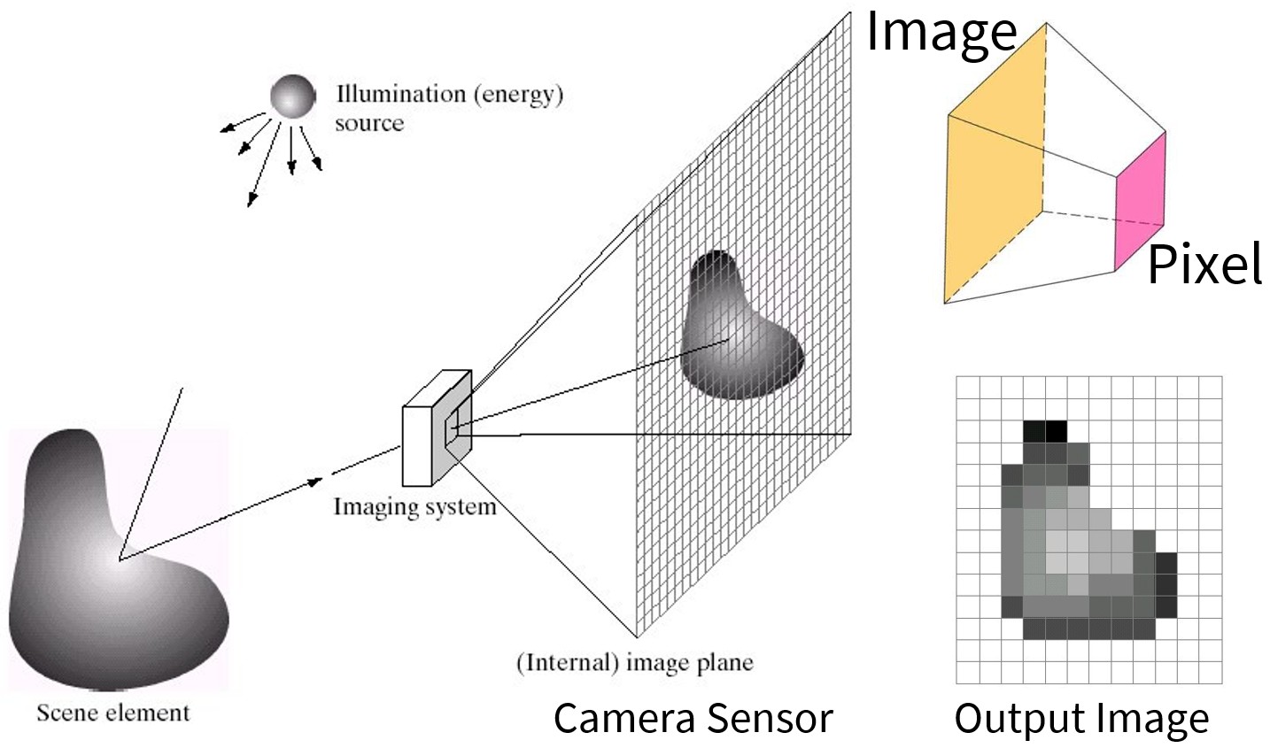
The imaging pipeline converts a continuous physical signal into discrete sensor measurements.
Sampling in Practice: Digital Image
Scene / image plane
Light signal
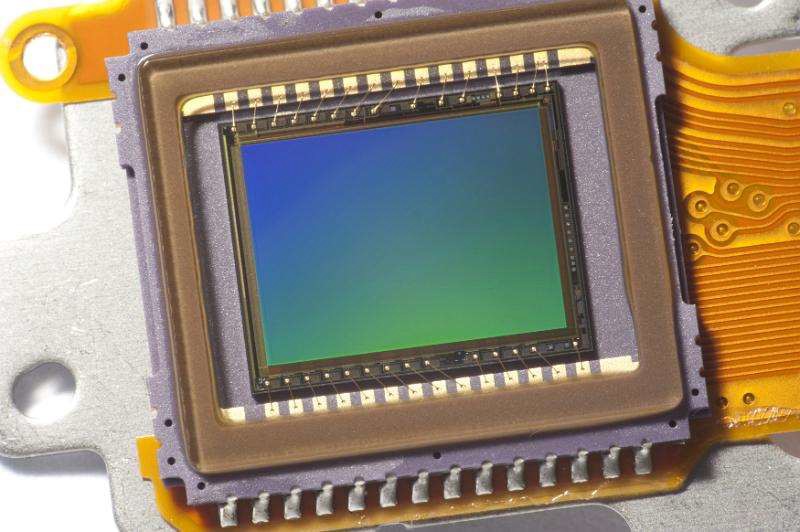
CMOS / CCD sensor
Digital cameras use sensor arrays to sample light and produce a grid of pixel values.
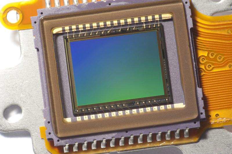
Sensor Array
Camera / sensor hardware
CMOS sensor array
Continuous light is sampled and quantized by the 2D sensor array (pixels) to produce a digital image.
Elements of a Digital Image
A pixel is a picture element.
For a grayscale image:
\[
I(x, y) = \text{intensity at image location} (x,y)
\]
\(x\): horizontal coordinate
\(y\): vertical coordinate
Example:
I(x1, y1) = 101I(x2, y2) = 191
Different pixel locations can have different intensity values.
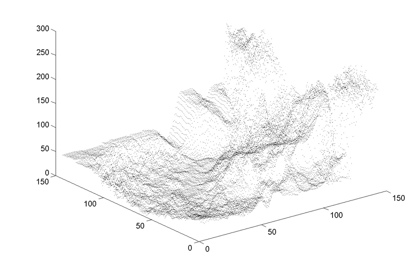
Digital Image is a 2D Signal
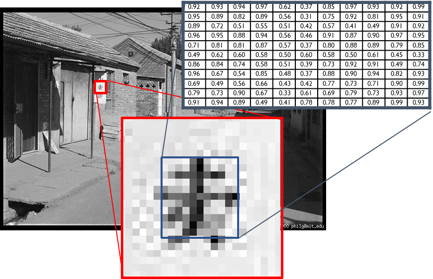
A digital image can be interpreted as a 2D function whose value is brightness or intensity.
Light Integration Over a Pixel Region
A single pixel does not measure an infinitely thin ray.
It measures light integrated over a small region of the sensor and the corresponding cone/frustum of incoming light.
Note
This is one reason why cameras blur, average, and alias details that are smaller than a pixel can represent.
Resolution: Geometric vs. Spatial
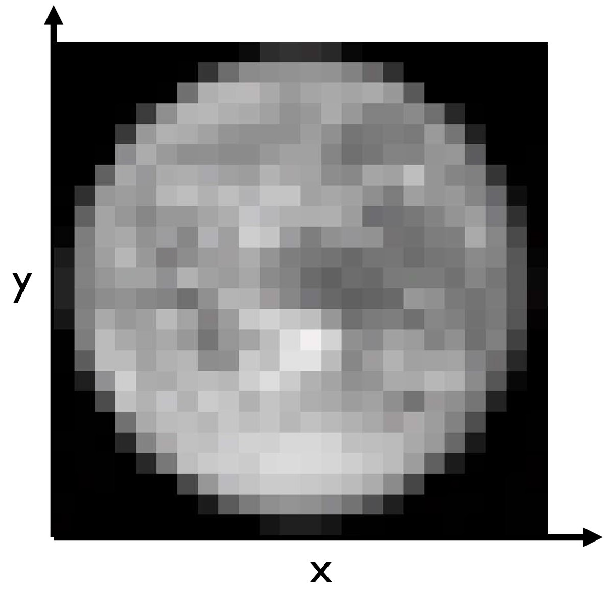
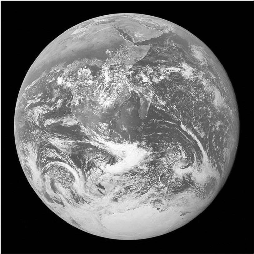
Both images can have the same number of pixels, but the amount of scene detail represented can be different.
Low geometric resolution
High geometric resolution
Note
Spatial resolution counts pixels. Geometric resolution is how accurately those pixels represent the positions of objects in the real world; or how sharp the image is. Geometric resolution is limited by physics, optics, and the environment (see Rayleigh criterion).
Quantization
Sampling chooses where to measure a signal.
Quantization chooses which values can be represented.
For example, an 3 bits can represent: \[
2^3 = 8
\] possible intensity levels in a grayscale image.
Quantization Effects — Radiometric Resolution
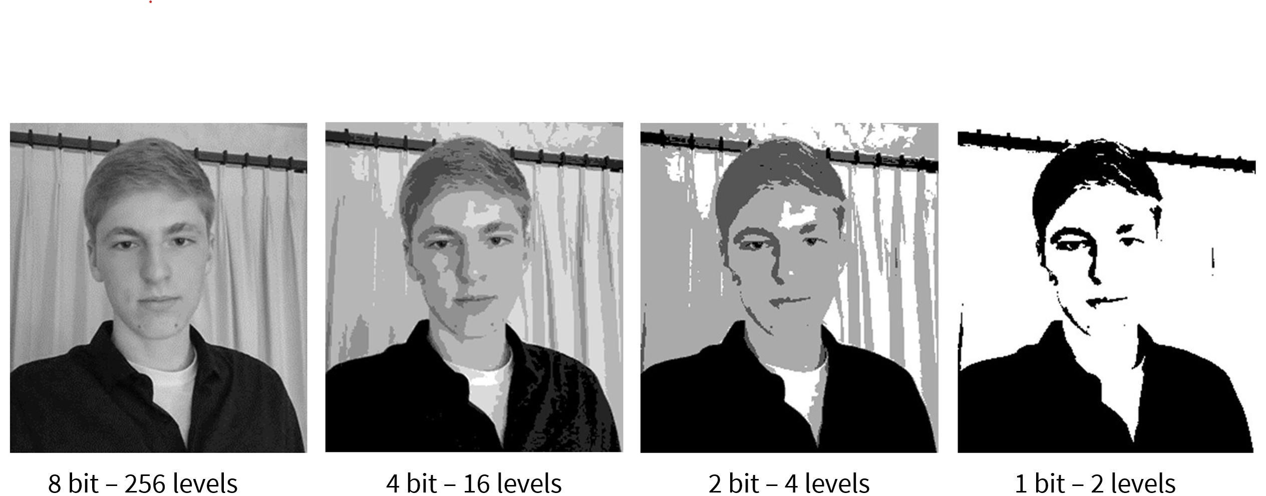
Radiometric resolution is the number of distinct intensity levels available.
Bit depth
Number of levels
1 bit
2 levels
2 bit
4 levels
4 bit
16 levels
8 bit
256 levels
Higher bit depth can represent more subtle intensity differences.
In photography, this is closely related to dynamic range.
Dimensionality of an Image
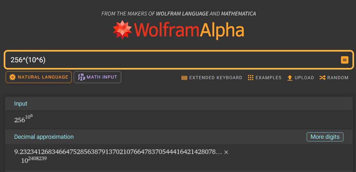
An image of size \(1000 \times 1000\) with 8-bit quantization per pixel has: \[
256^{1000 \times 1000} \approx 10^{2,408,239}
\] possible intensity configurations.
This is an enormous high-dimensional space – the known universe has only about \(10^{80}\) atoms!
Computer vision works in this extremely high dimensional space – but real images are not arbitrary arrays and they occupy a small, structured subset of this space.
Images in Python: Grayscale Arrays
For an \(N \times M\) grayscale image im:
im[0, 0] # top-left pixel valueim[y, x] # y rows down, x columns rightim[N-1, M-1] # bottom-right pixel value
Important
In NumPy, image indexing is usually row first, column second: im[y, x], not im[x, y].
Grayscale Intensity
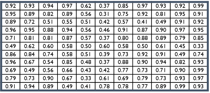
A grayscale image is a matrix that stores one intensity value per pixel.
Color Images
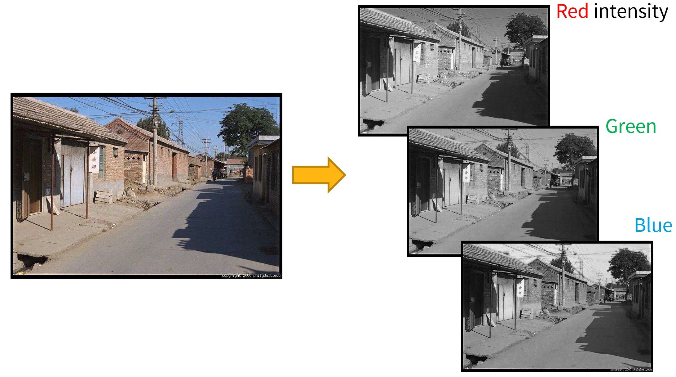
A color image stores multiple intensity values per pixel.
For RGB images, each pixel has three channels:
Red intensity
Green intensity
Blue intensity
image shape: height × width × 3
Note
Different libraries may use different channel order conventions. OpenCV commonly uses BGR; Matplotlib commonly expects RGB.
Images in Python: Color Arrays
For an \(N \times M\) color image im with three channels:
im[0, 0, 0] # top-left pixel, first channelim[y, x, 1] # pixel at row y, column x, second channelim[N-1, M-1, 2] # bottom-right pixel, third channel
Typical shape:
im.shape # (height, width, channels)
For an RGB image:
channel 0 = redchannel 1 = greenchannel 2 = blue
For OpenCV-loaded images:
channel 0 = bluechannel 1 = greenchannel 2 = red
Images in Python: Data Types
Take care of image data types.
# uint8 image: values 0 to 255im = cv2.imread("file.jpg")# convert to float32, still values 0 to 255im_float = im.astype(np.float32)# normalize to 0 to 1im_norm = im.astype(np.float32) /255.0
Important
Many image-processing bugs come from mixing uint8, float32, and different value ranges.
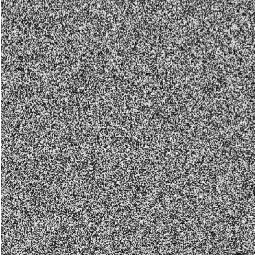
Random Images in Python
from numpy import random as rI = r.rand(256, 256)
r.rand(256, 256) creates a 256 by 256 array of random floating-point values in the range \([0,1)\).
Questions:
What is I?
What does it look like?
Which values does it contain?
How many values are there?
Displaying an Image in Python
from matplotlib import pyplot as pltfrom numpy import random as rI = r.rand(256, 256)plt.imshow(I, cmap="gray")plt.axis("off")plt.show()
Is this an image?
Coding in This Course
We will use:
Python for programming
Conda for managing the course environment
NumPy for numerical arrays
OpenCV for image processing and computer vision
PyTorch for deep learning topics
VS Code for editing, debugging, and notebooks
Important
Do not use GenAI to solve homework for you. If you copy-paste code without understanding it, you will not learn how to code.
Be kind and supportive: students come from different backgrounds and have different levels of Python experience.
 Blue Marble, NASA / Apollo 17
 Scene / object
 Light as a signal
 Camera / sensor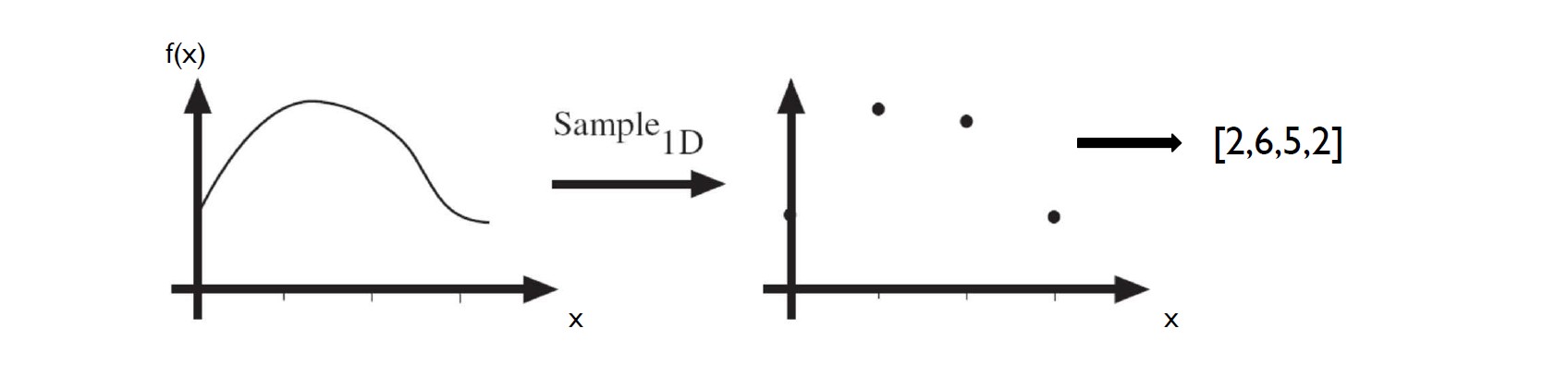
 World / scene
 Scene / image plane
 CMOS / CCD sensor
 Camera / sensor hardware
 CMOS sensor array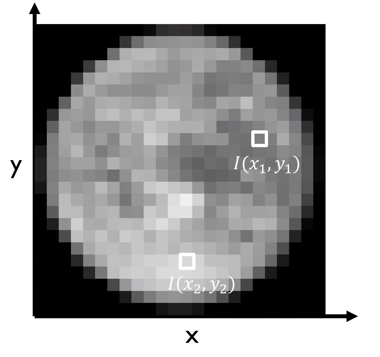
 Low geometric resolution
 High geometric resolution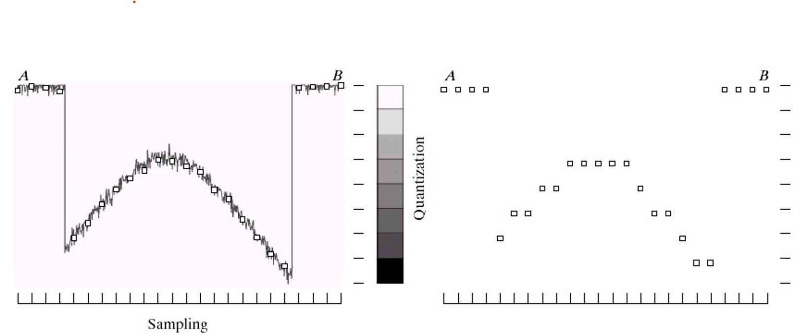
 Is this an image?