Lecture 03 — Image Filtering
Lecture 3
Image Filtering
Filtering Modifies a Signal
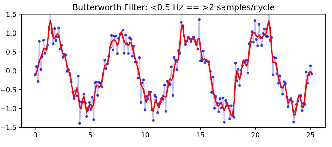 Noisy samples and a smoothed estimate
Filtering transforms a signal to:
- suppress undesired components such as noise
- emphasize useful structure
- extract specific features
Filters can operate on continuous or discrete signals in one or more dimensions.
1D Moving Average Filter
For a window size \(k\):
\[ y[n] = \frac{1}{k} \sum_{i=n-k+1}^{n} (1) I[i] \qquad \qquad \text{or} \qquad \qquad y[n] = \frac{1}{k} \begin{bmatrix} 1 & 1 & \cdots & 1 \end{bmatrix} \begin{bmatrix} I[n-k+1] \\ I[n-k+2] \\ \vdots \\ I[n] \end{bmatrix} \]
x = np.linspace(0, 4*np.pi, 160)
rng = np.random.default_rng(7)
noisy = np.sin(x) + 0.28*rng.normal(size=x.size)

k = 10
ker = np.ones(k)/k
smoothed = np.convolve(noisy, ker, mode="full")[:noisy.size]

fig, ax = plt.subplots(figsize=(6.5, 3.5))
ax.plot(x, noisy, c="0.65", lw=2, label="Signal")
ax.plot(x, smoothed, c="blue", lw=3, label="Moving average")
ax.set(xlabel="$x$", ylabel="Value")
ax.legend(frameon=False); ax.grid(alpha=0.2)
plt.tight_layout(); plt.show()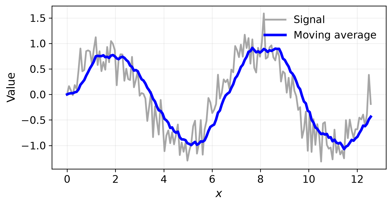
The Window Size \(k\)
A larger averaging window:
- removes more rapid variation
- produces a smoother output
- spreads changes over a wider region
- can erase narrow but meaningful features
x = np.linspace(0, 4*np.pi, 160)
rng = np.random.default_rng(7)
noisy = np.sin(x) + 0.28*rng.normal(size=x.size)

k = 50
ker = np.ones(k)/k
smoothed = np.convolve(noisy, ker, mode="full")[:noisy.size]

fig, ax = plt.subplots(figsize=(6.5, 3.5))
ax.plot(x, noisy, c="0.65", lw=2, label="Signal")
ax.plot(x, smoothed, c="blue", lw=3, label="Moving average")
ax.set(xlabel="$x$", ylabel="Value")
ax.legend(frameon=False); ax.grid(alpha=0.2)
plt.tight_layout(); plt.show()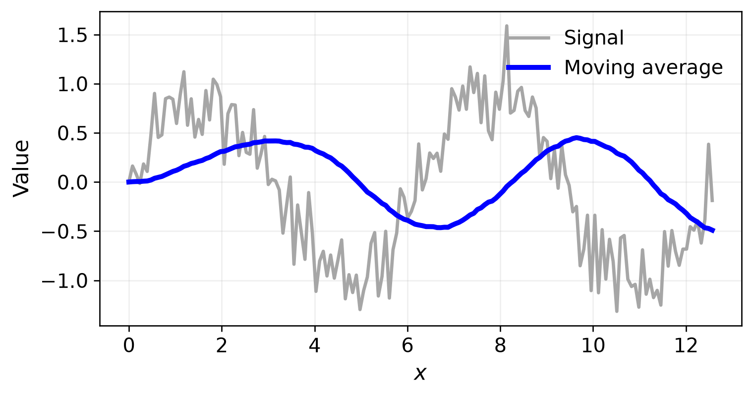
Filter Kernel
What is this filter doing?
\[ y[n] = \begin{bmatrix} 0 & 0 & \cdots & 0 & 1 \end{bmatrix} \begin{bmatrix} I[n-k+1] \\ I[n-k+2] \\ \vdots \\ I[n] \end{bmatrix} \]
x = np.linspace(0, 4*np.pi, 160)
rng = np.random.default_rng(7)
noisy = np.sin(x) + 0.28*rng.normal(size=x.size)

k = 20
ker = np.zeros(k); ker[-1] = 1
output = np.correlate(np.pad(noisy, (k-1, 0)), ker, mode="valid")

fig, ax = plt.subplots(figsize=(6.5, 3.5))
ax.plot(x, noisy, c="0.65", lw=4, label="Input")
ax.plot(x, output, "b--", lw=2.5, label="Output")
ax.set(xlabel="$x$", ylabel="Value")
ax.legend(frameon=False); ax.grid(alpha=0.2)
plt.tight_layout(); plt.show()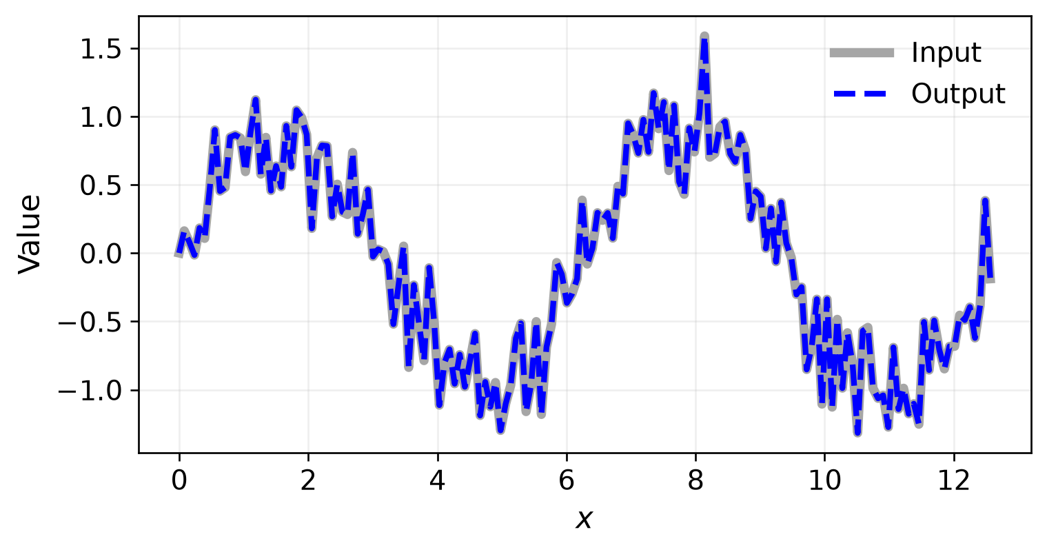
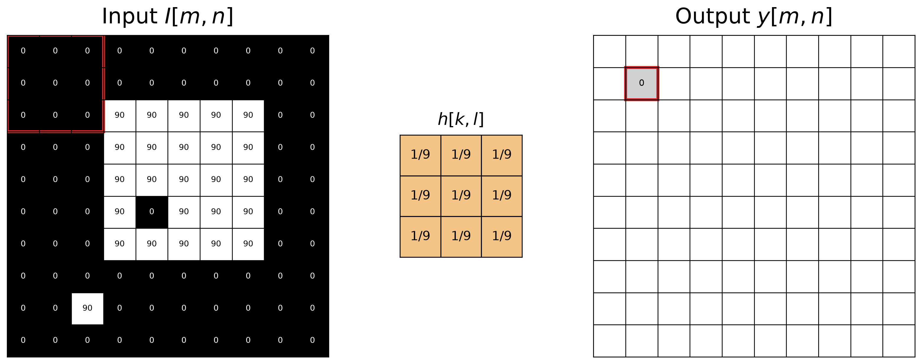
Box Filter: Move One Pixel Right
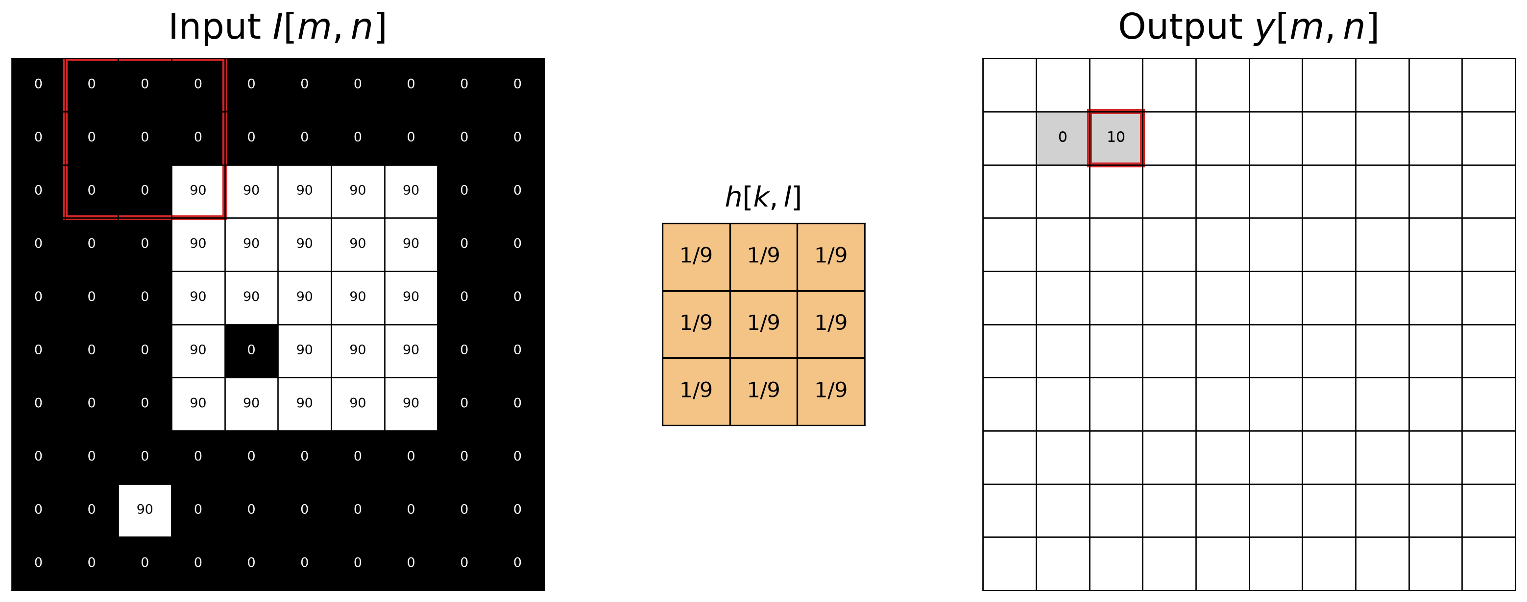
\[ y[1,2]=\sum_{k=-1}^{1}\sum_{l=-1}^{1}h[k,l]I[1+k,2+l]=10 \]
Box Filter: Continue the Sweep
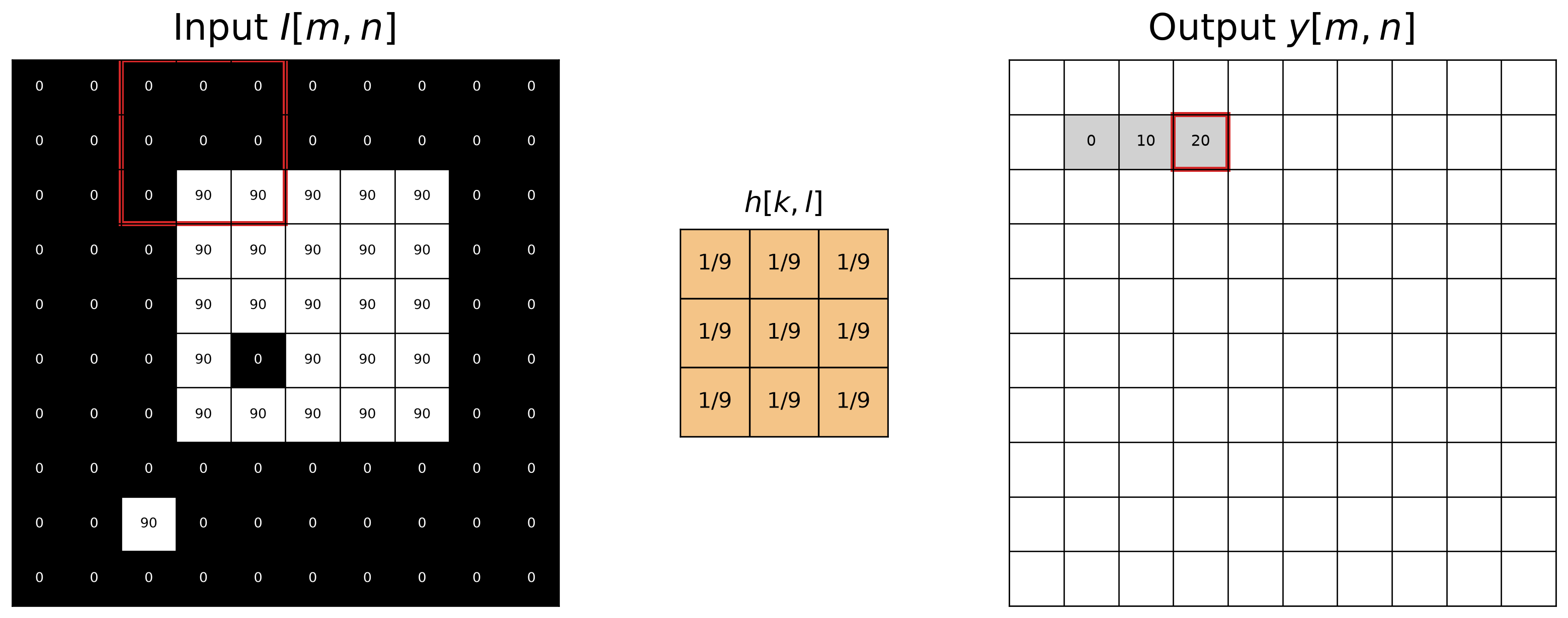
\[ y[1,3]=\sum_{k=-1}^{1}\sum_{l=-1}^{1}h[k,l]I[1+k,3+l]=20 \]
Box Filter: Continue the Sweep
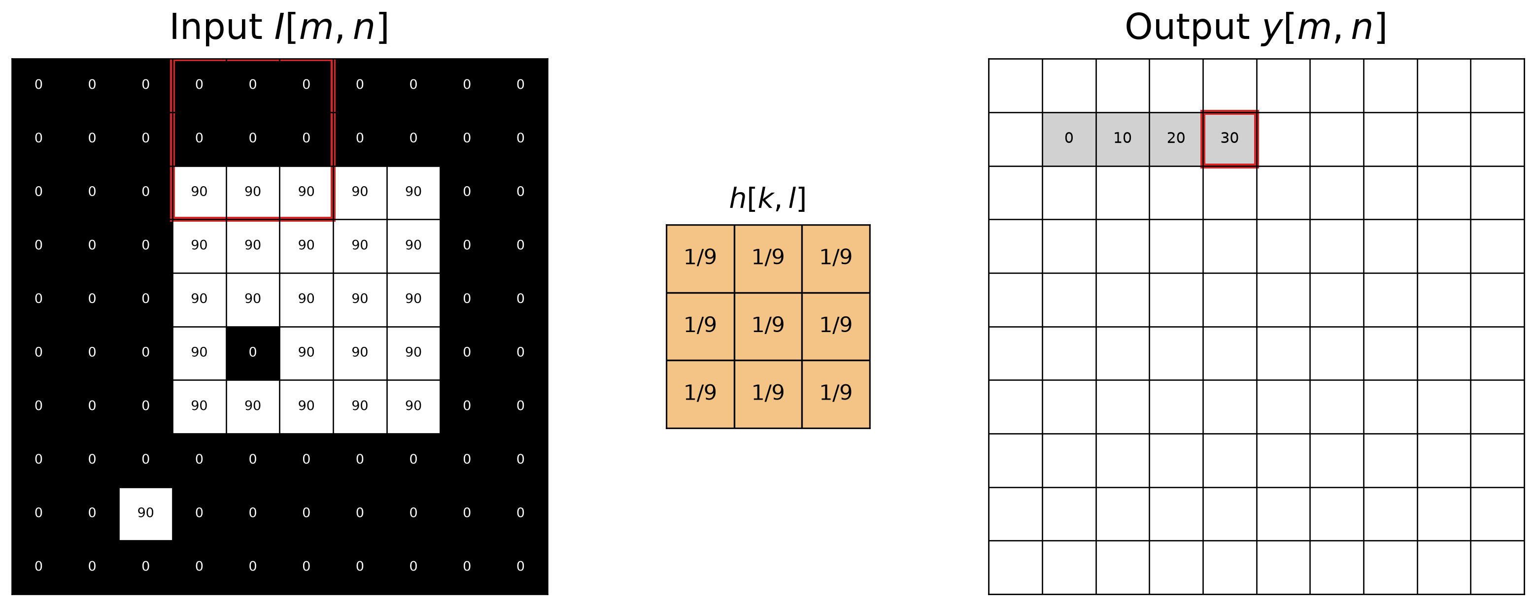
\[ y[1,4]=\sum_{k=-1}^{1}\sum_{l=-1}^{1}h[k,l]I[1+k,4+l]=30 \]
Box Filter: Continue the Sweep
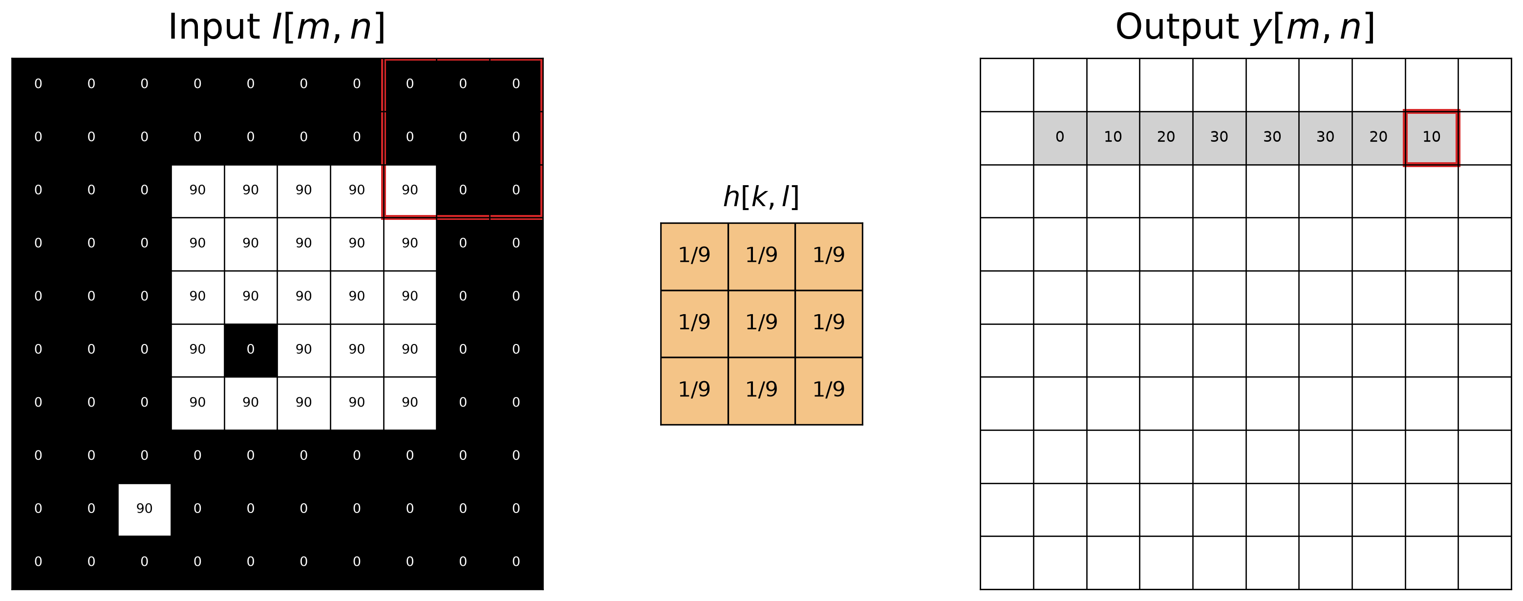
\[ y[1,8]=\sum_{k=-1}^{1}\sum_{l=-1}^{1}h[k,l]I[1+k,8+l]=10 \]
Box Filter: Continue Across the Column
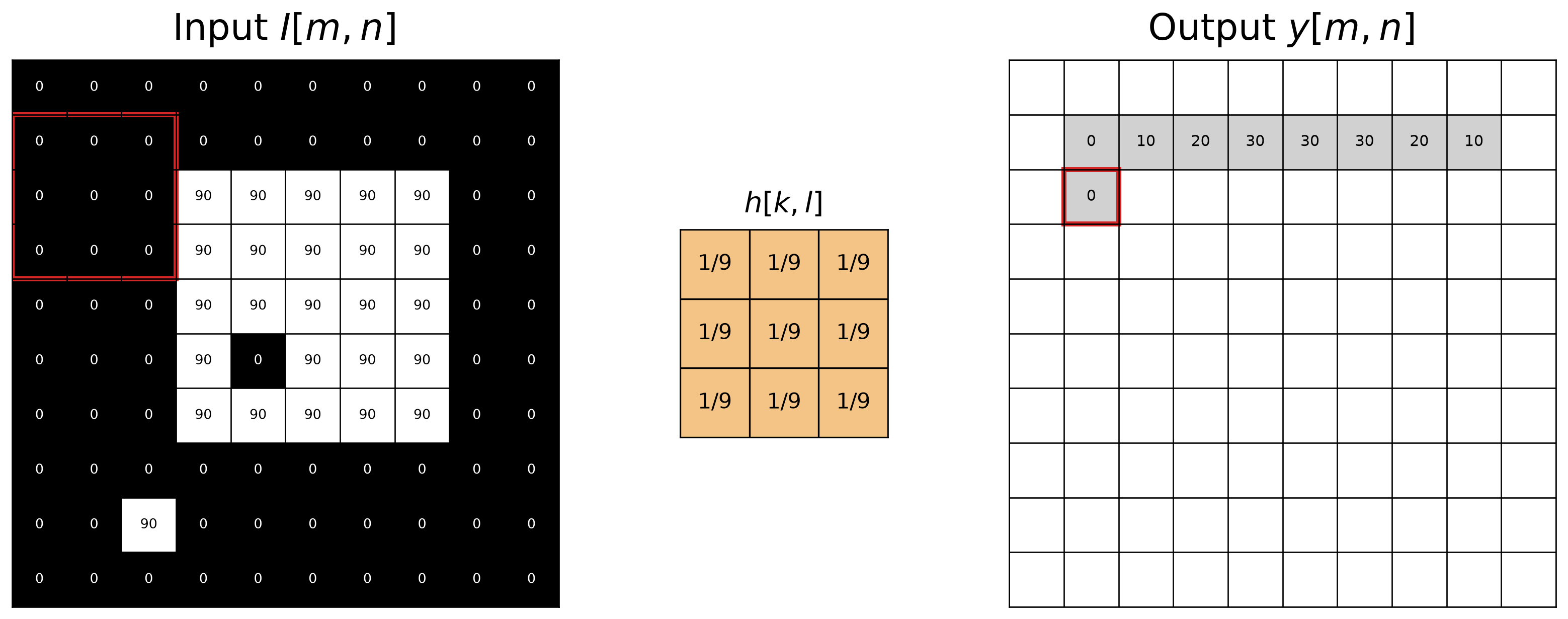
\[ y[2,1]=\sum_{k=-1}^{1}\sum_{l=-1}^{1}h[k,l]I[2+k,1+l]=0 \]
Box Filter: Try This Position
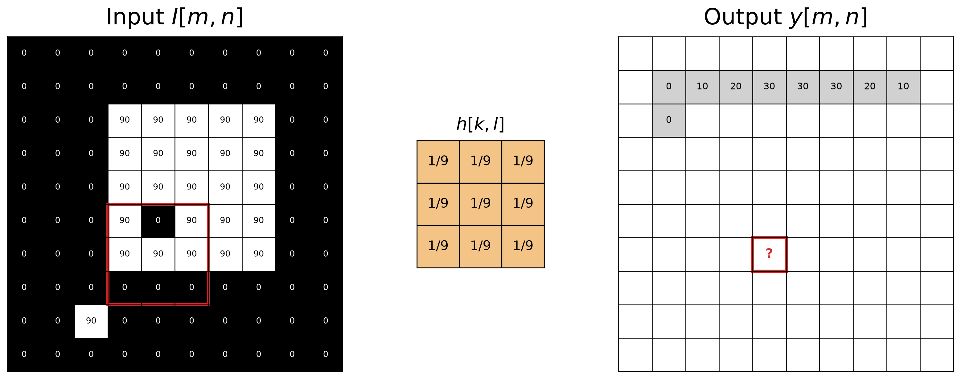
What is \(y[6,4]\)?
Add the nine pixels under the red window, then divide by nine.
Box Filter: Another Position
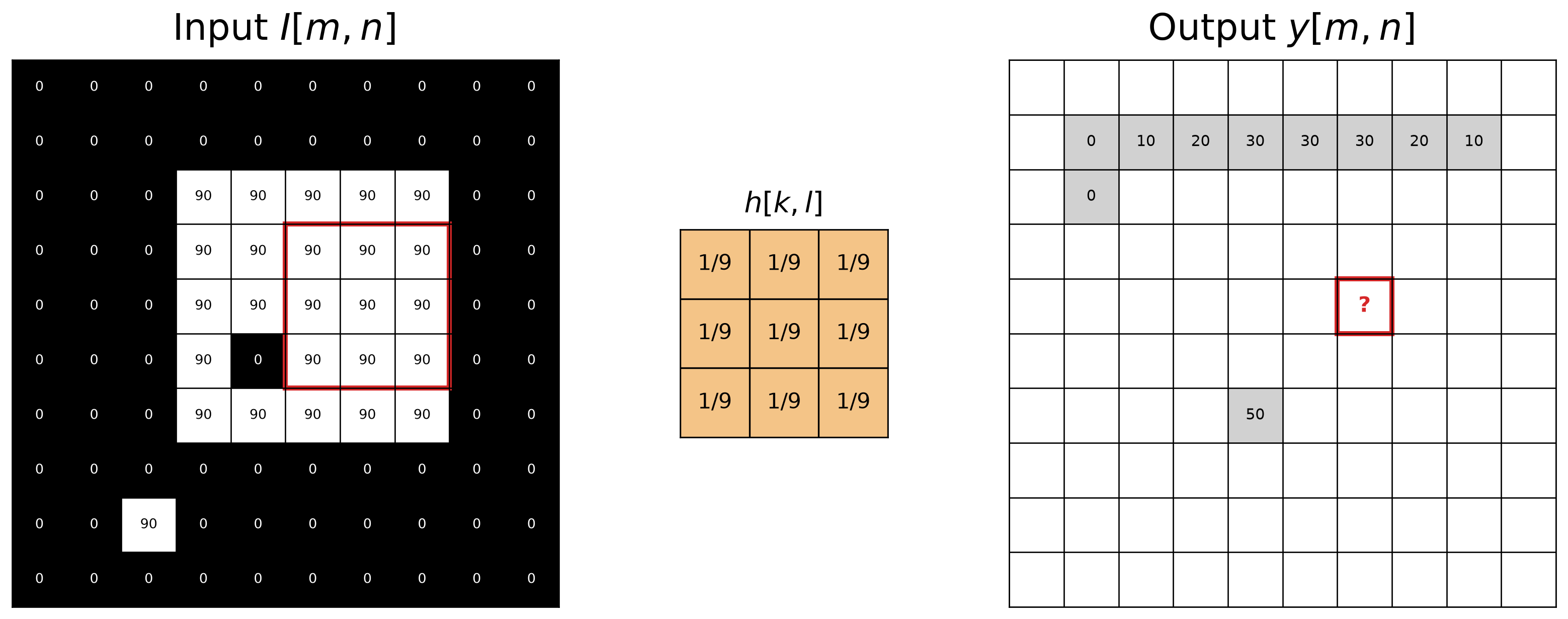
What is \(y[4,6]\)?
Box Filter: Complete Output
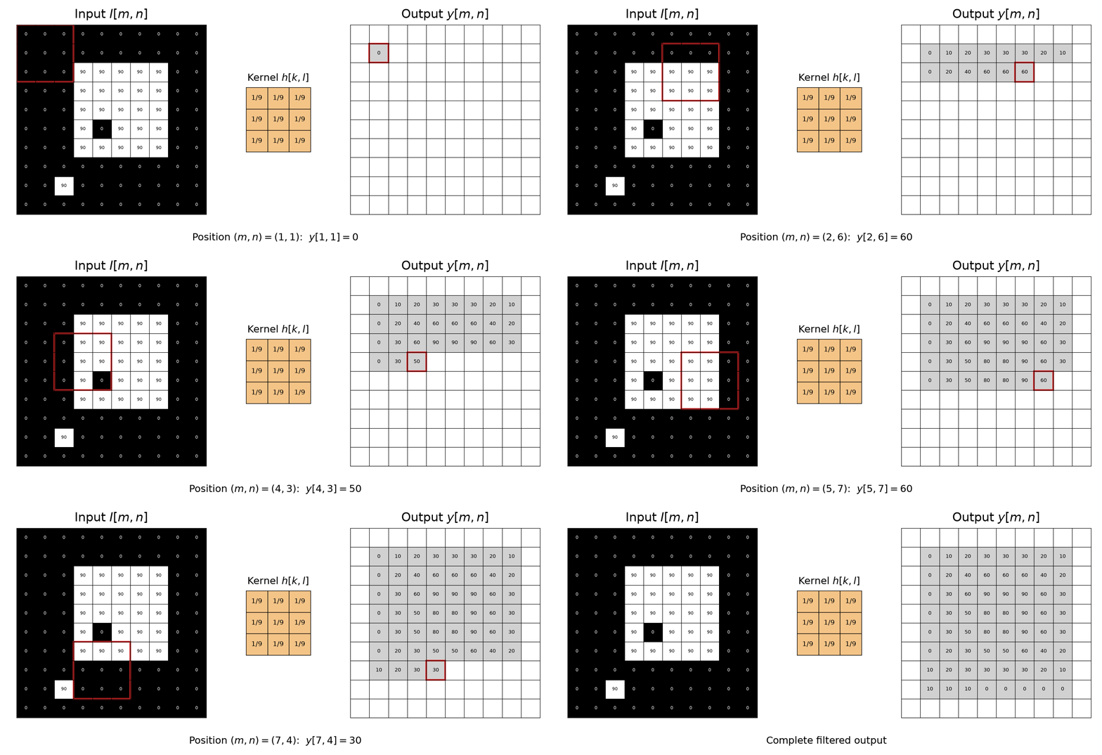
Box Filter: Complete Output
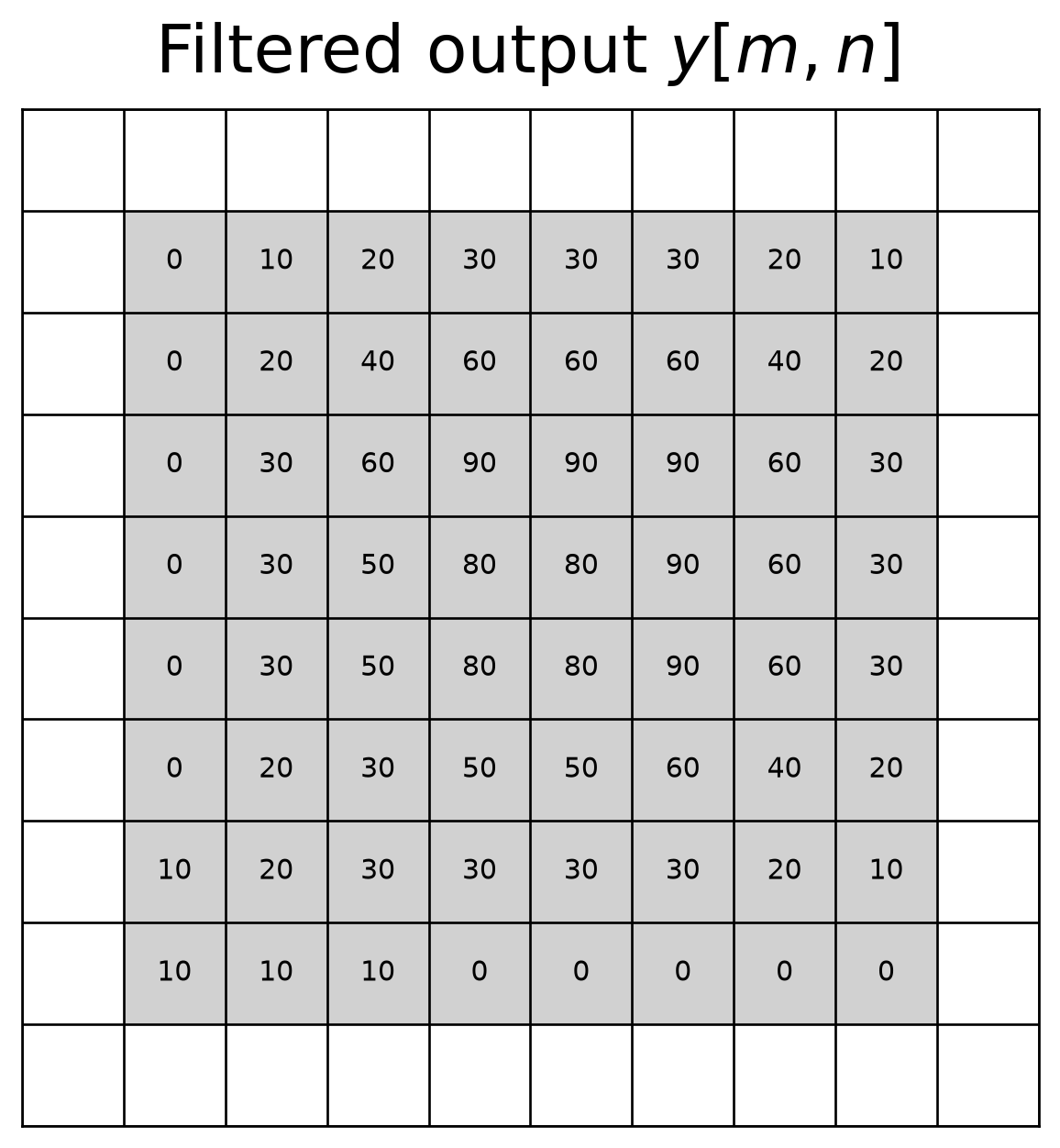
\[ y[m,n]=\sum_{k=-1}^{1}\sum_{l=-1}^{1}h[k,l]I[m+k,n+l] \]
Smoothing with a Box Filter
- For a \(k\times k\) box filter, \(h[k,k]=1/k^2\).
- A larger \(k\) produces stronger smoothing
import cv2

img_path = Path("assets/03_filtering/bloom_original.jpg")
img_col = cv2.imread(str(img_path))

img_gray = cv2.cvtColor(img_col, cv2.COLOR_BGR2GRAY)
img_flt = img_gray.astype(np.float32) / 255.0
img = cv2.resize(img_flt, None, fx=0.2, fy=0.2)

box3 = cv2.blur(img, (3, 3), borderType=cv2.BORDER_CONSTANT)
box9 = cv2.blur(img, (9, 9), borderType=cv2.BORDER_CONSTANT)

fig, axes = plt.subplots(1, 3, figsize=(6.5, 3))
for ax, result, title in zip(
    axes, [img, box3, box9], ["Original", "$k=3$", "$k=9$"]):
    ax.imshow(result, cmap="gray", vmin=0, vmax=1)
    ax.set_title(title); ax.axis("off")
plt.tight_layout(pad=0.5)
plt.show()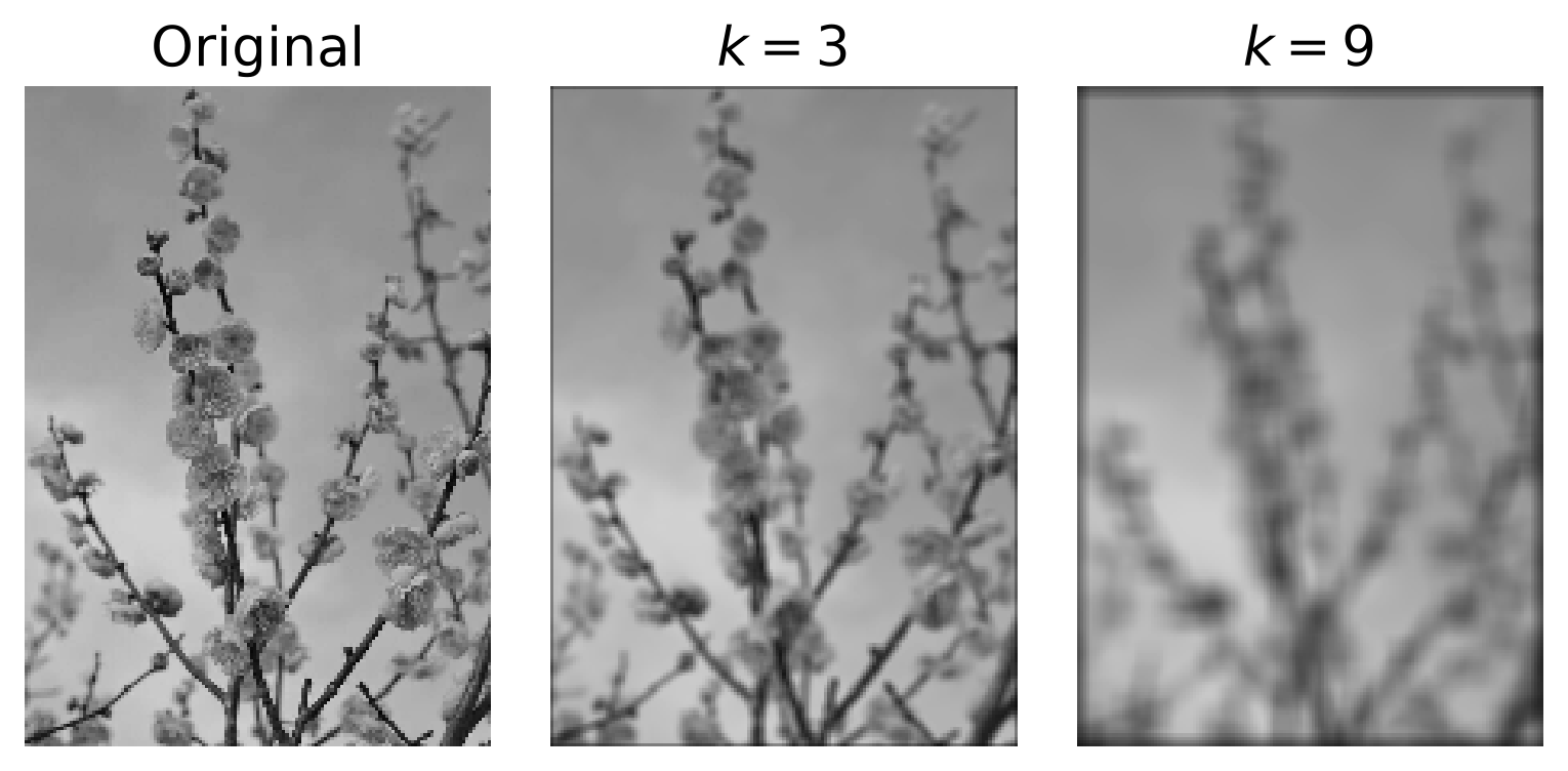
Gaussian Filter Kernel
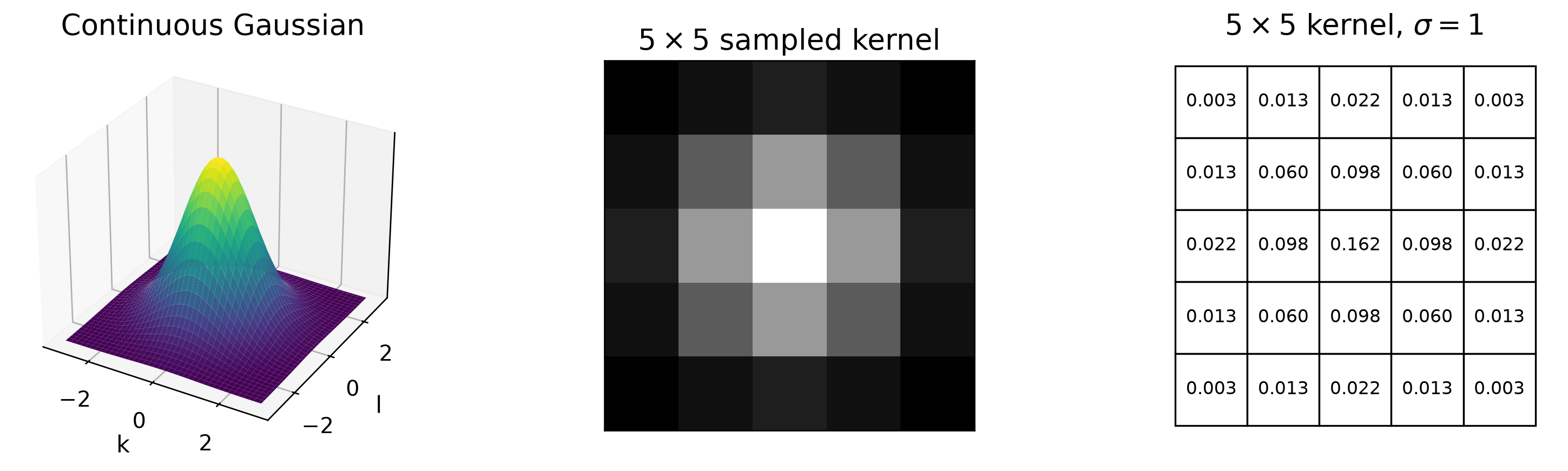
A Gaussian kernel gives the largest weight to the center pixel and smoothly decreases with distance:
\[ h_\sigma[k,l] = \frac{1}{2\pi\sigma^2} \exp\left(-\frac{k^2+l^2}{2\sigma^2}\right). \]
Gaussian Filter Kernel
Note
- Gaussian kernel weights sums to one (aside from negligible floating-point errors) – why?
- The continuous Gaussian integrates to one over the infinite plane. A truncated (5) sample does not automatically sum to one, so the explicit normalization line is necessary.
- Sampled kernel size should be large enough to include the meaningful support of the Gaussian—often several standard deviations on each side.
Smoothing with a Gaussian Filter
- A Gaussian filter smooths noises.
import cv2

gau3 = cv2.GaussianBlur(img, (3, 3), sigmaX=0, borderType=cv2.BORDER_CONSTANT)
gau9 = cv2.GaussianBlur(img, (9, 9), sigmaX=0, borderType=cv2.BORDER_CONSTANT)

fig, axes = plt.subplots(1, 3, figsize=(6.5, 5))
for ax, im, title in zip(
    axes, [img, gau3, gau9],
    ["Original", r"Gaussian ($k=3$)", r"Gaussian ($k=9$)"]):
    ax.imshow(im, cmap="gray", vmin=0, vmax=1)
    ax.set_title(title)
    ax.axis("off")
plt.tight_layout(pad=0.3)
plt.show()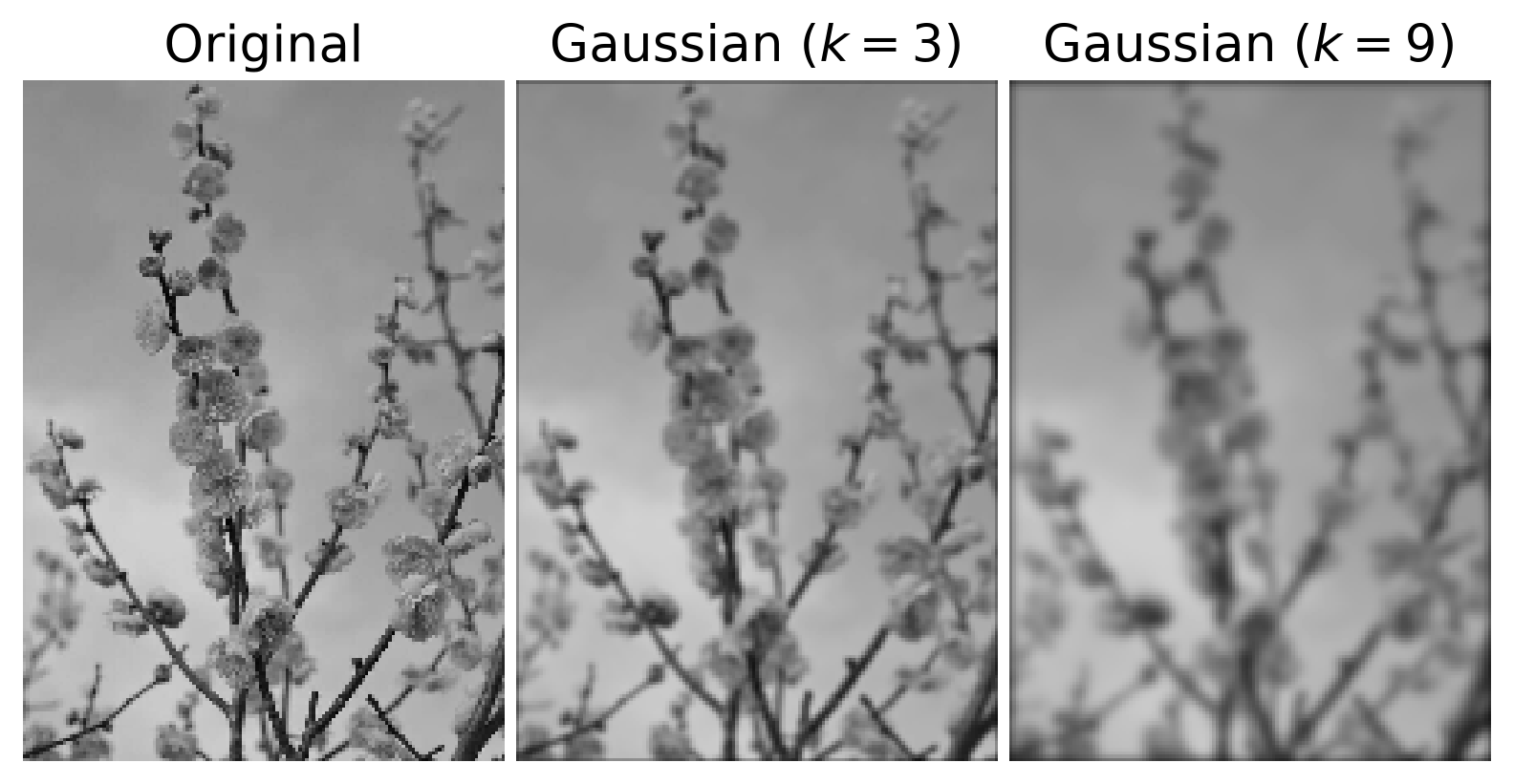
Box versus Gaussian Filter Smoothing
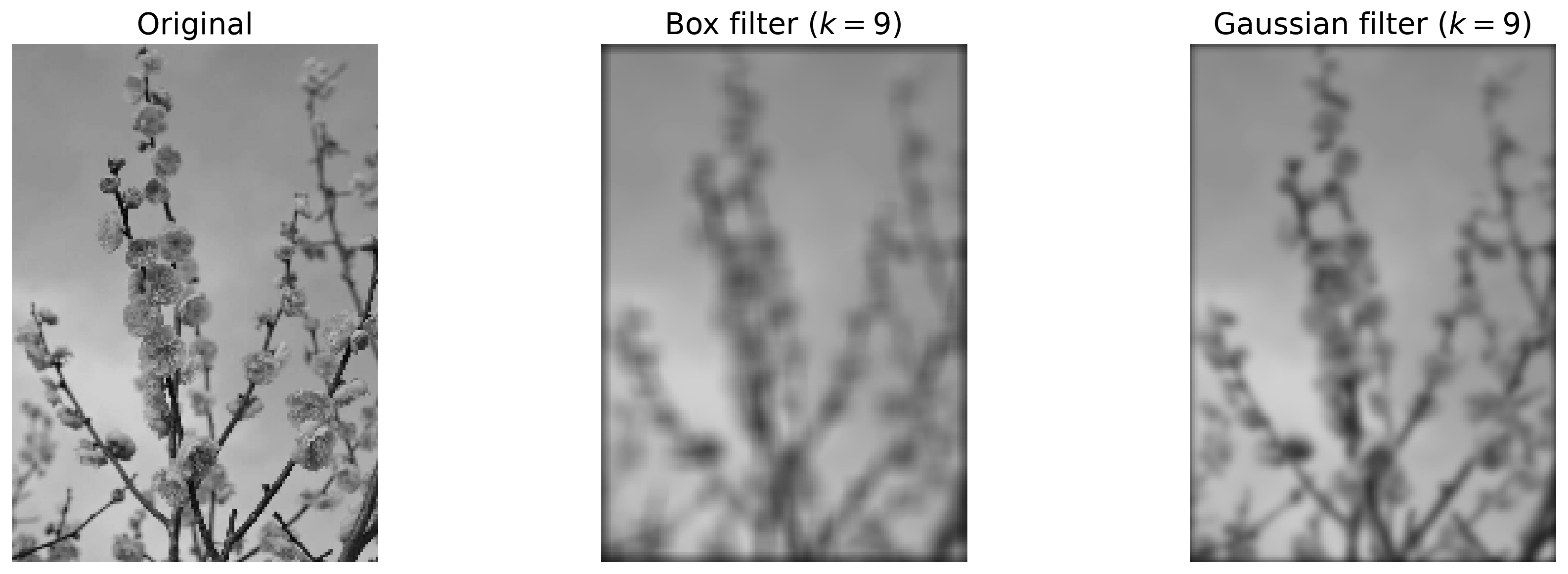
- The box filter weights every pixel in the window equally.
- The Gaussian filter changes weights smoothly, which produces fewer artifacts.
Linear Filter Properties
Linearity:
\[ \text{filter}(I, h_1 + h_2)=\text{filter}(I, h_1)+\text{filter}(I, h_2) \]
Shift/translation invariance:
\[ \text{filter}(I, \text{shift}(h))= \text{shift}(\text{filter}(I, h)) \]
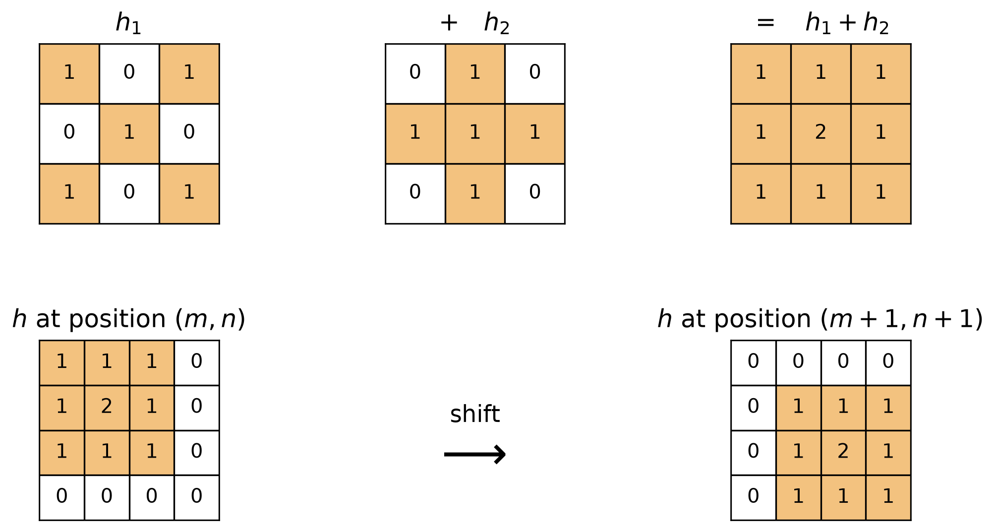
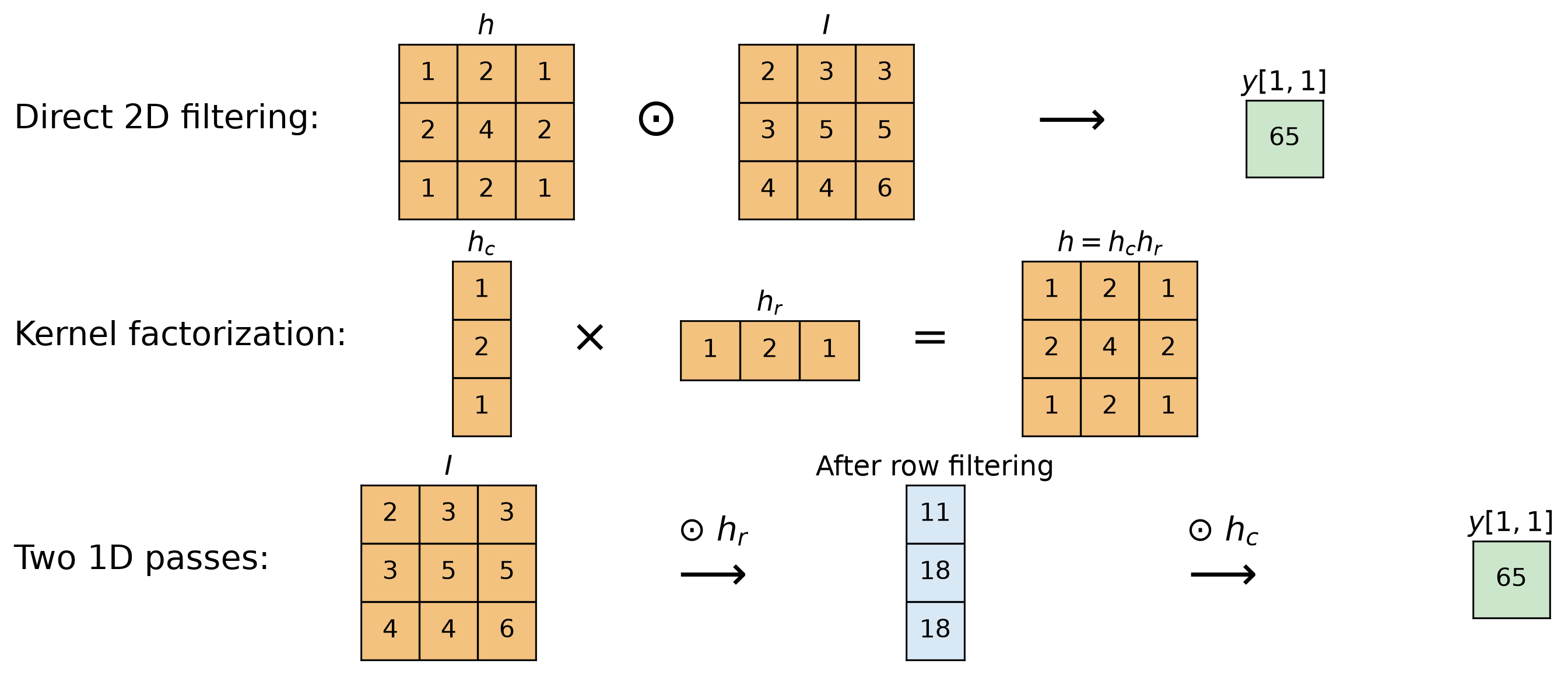
Separability Example
Correlation and Convolution Differ for Asymmetric Kernels
A kernel rotated by \(180^\circ\): \(\widetilde{h}[k,l]=h[-k,-l]\).
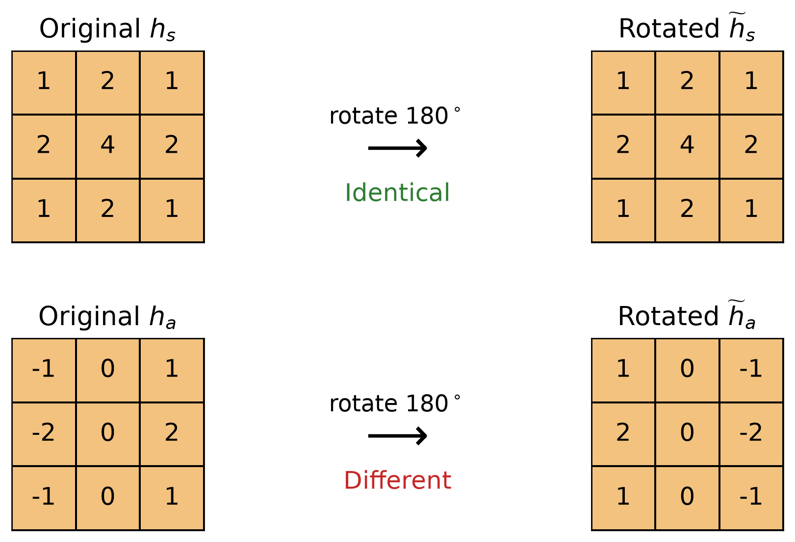
- Since \(h_s=\widetilde{h}_s\), correlation and convolution produce the same result.
- But \(h_a\neq\widetilde{h}_a\), so correlation and convolution produce different responses.
“Convolution” Layers Usually Compute Correlation
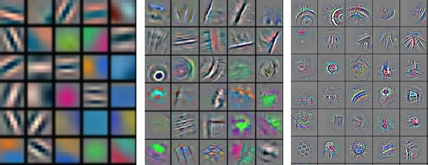
- Convolutional neural networks learn their kernel weights from data rather than using predefined filters.
- Despite the name, most deep-learning libraries apply learned kernels without rotating them, which is, correlation.
- This does not reduce the network’s expressive power since the kernel is learned, and the network can learn either a kernel or its rotated version.
Boundary Handling
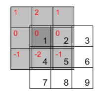
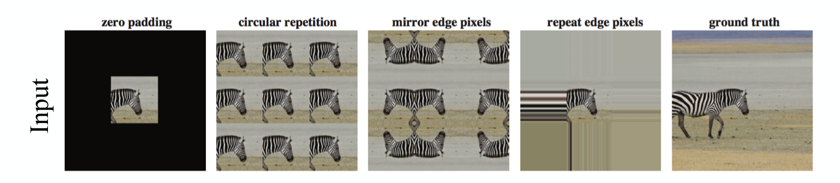
Near an image boundary, part of the kernel falls outside the available data. Need to extrapolate (padding) to compute the output edge pixels.
| Strategy | Assumption outside the image | Common consequence |
|---|---|---|
| Constant / zero | Missing pixels have a fixed value | Dark or bright border artifacts |
| Replicate | Repeat the closest boundary pixel | Flat extension at the edge |
| Reflect | Mirror the image across the boundary | Often smoothest for natural images |
| Wrap | Opposite edges are adjacent | Appropriate for periodic data |
| Valid only | Skip incomplete neighborhoods | Smaller output image |
Note
Two implementations using the same kernel can disagree near the boundary if their padding modes differ.
Three Common Output Modes
import cv2

x = cv2.imread("assets/03_filtering/colorado-flower.jpg", 0)
x = cv2.resize(x, (200,120), interpolation=cv2.INTER_AREA).astype(np.float32)/255
h, w = x.shape

p = cv2.copyMakeBorder(x, h-1,0,w-1,0, cv2.BORDER_CONSTANT)
full = cv2.filter2D(p, cv2.CV_32F, x, anchor=(0,0), borderType=cv2.BORDER_CONSTANT)
same = cv2.filter2D(x, cv2.CV_32F, x, borderType=cv2.BORDER_CONSTANT)
valid = full[h-1:h, w-1:w]

ims, names = [x,full,same,valid], ["Input","full","same","valid"]
H, W = full.shape
fig, ax = plt.subplots(2,2,figsize=(6.5,5))

for a, im, name in zip(ax.flat, ims, names):
    ih, iw = im.shape
    a.imshow(im, cmap="gray", extent=(0,iw,ih,0), interpolation="nearest")
    a.set(xlim=(0,W), ylim=(H,0), title=fr"{name}: ${iw}\times{ih}$")
    a.axis("off")

plt.tight_layout(pad=.4)
plt.show()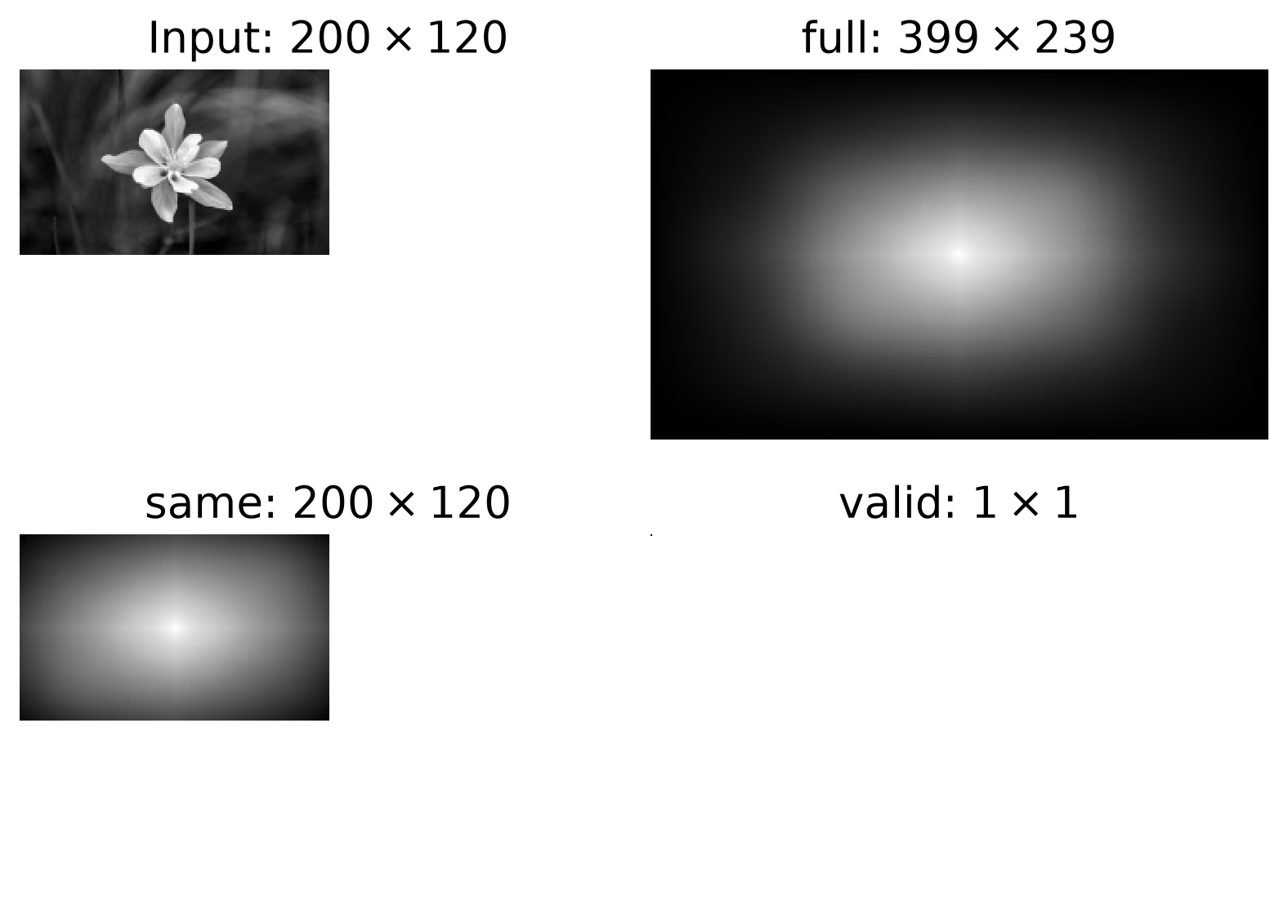
Practice with Linear Filters
Predict the effect of each kernel before viewing the following examples.
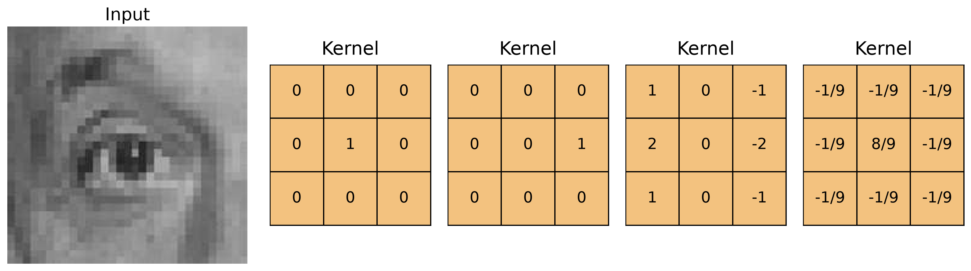
Practice:
What will this kernel do to the image?
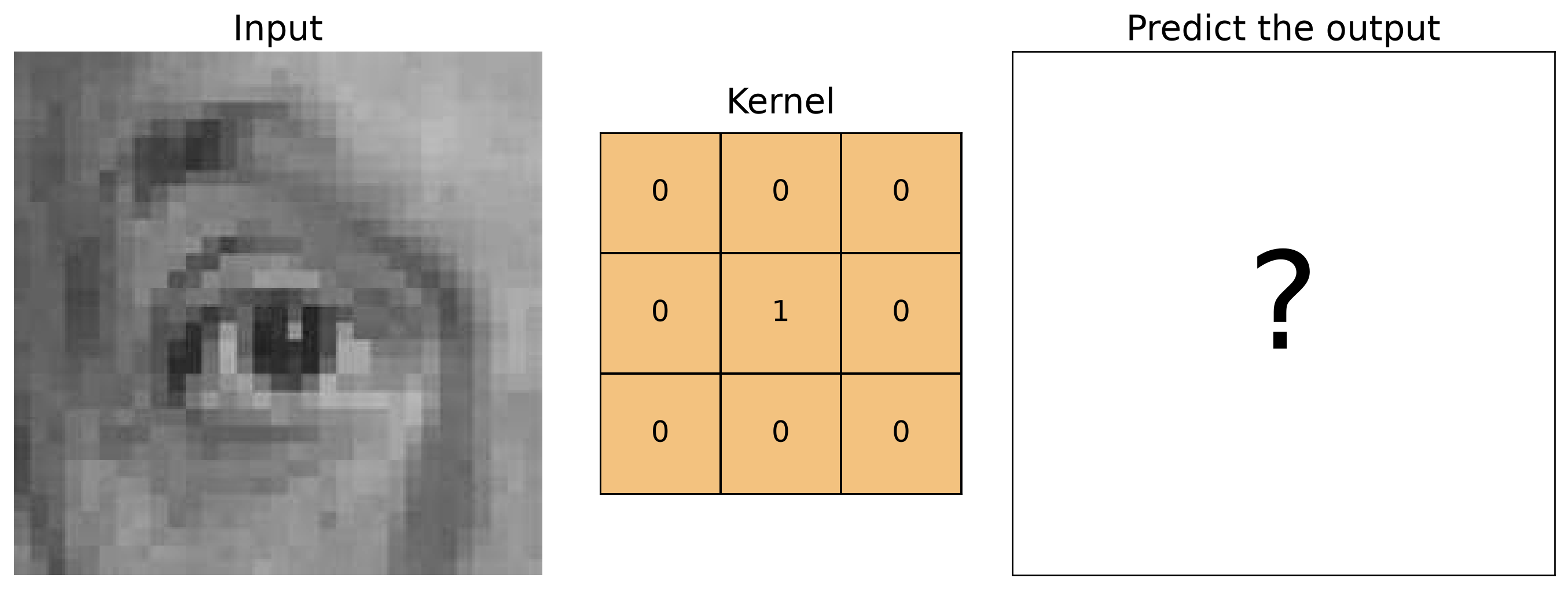
Identity Kernel Leaves the Image Unchanged
The center coefficient copies the current pixel:
\[ y[m,n]=I[m,n]. \]
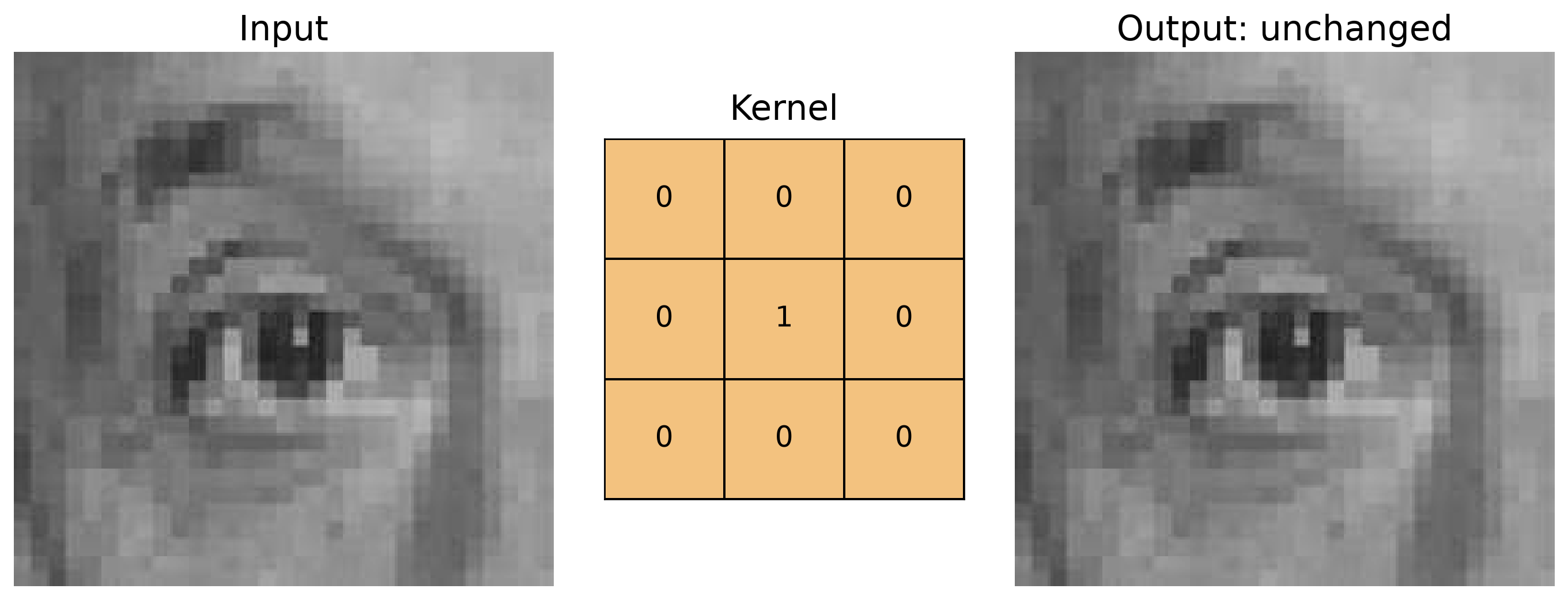
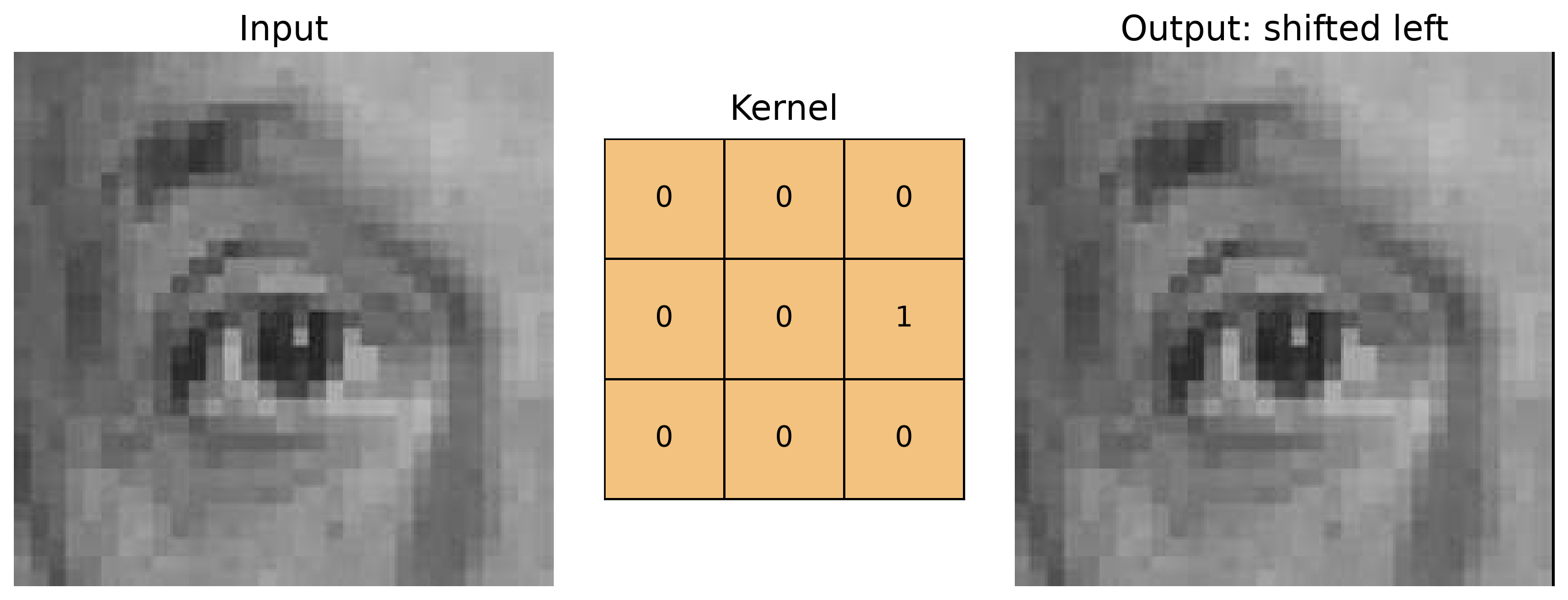
Practice:
What will happen when the kernel selects the pixel immediately to the right?
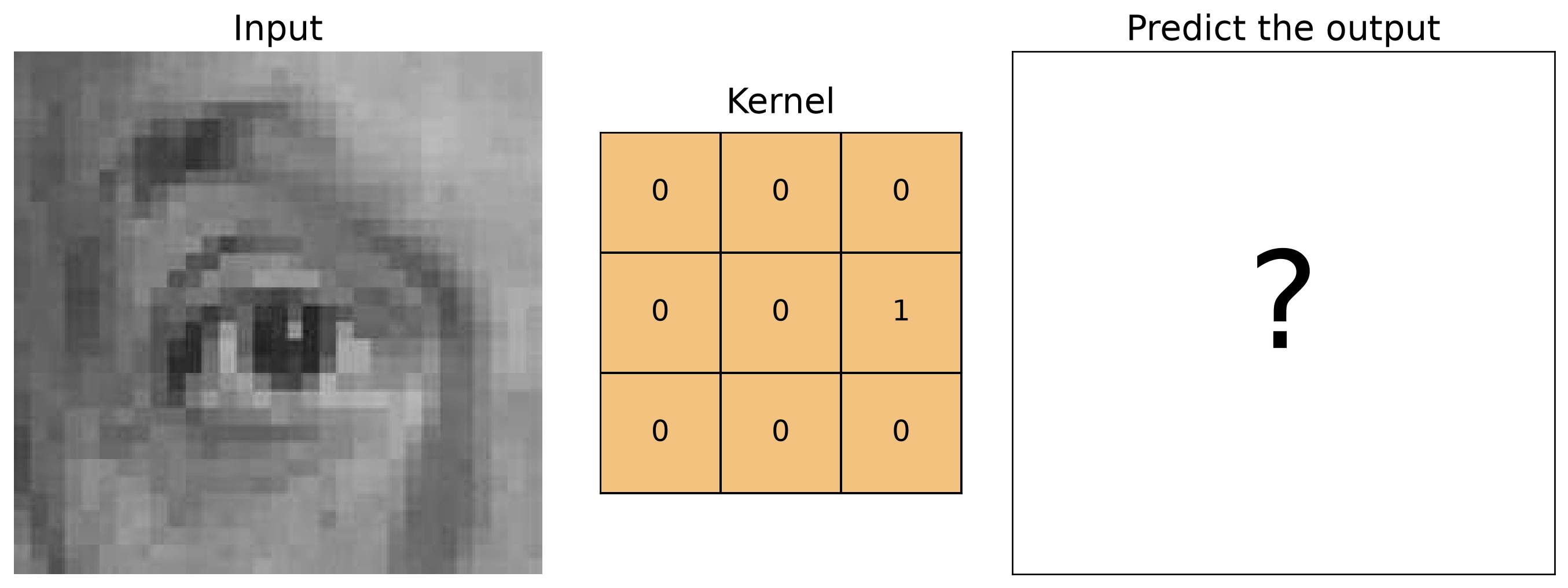
Shift Kernel Copies a Neighboring Pixel
For correlation, the kernel produces
\[ y[m,n]=I[m,n+1], \]
so the image content shifts left by one pixel.
Practice:
Examine the kernel and predict which image structures will produce the strongest response.
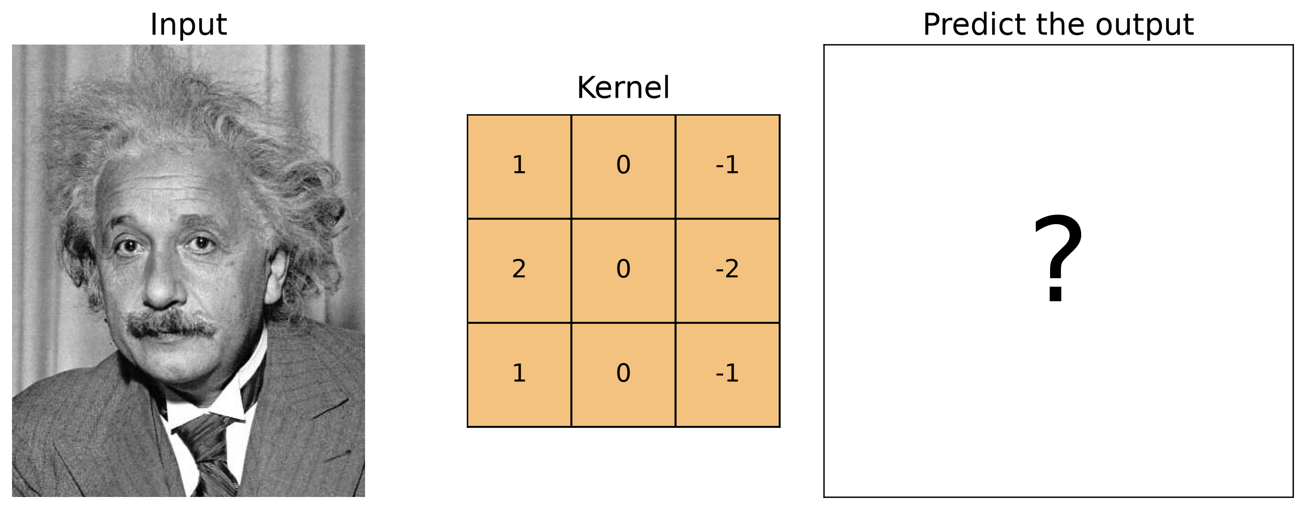
- Will the kernel respond to horizontal or vertical edges?
- Which regions of the image will have a response near zero?
Sobel \(x\): Detecting Vertical Edges
This kernel responds strongly to vertical edges.
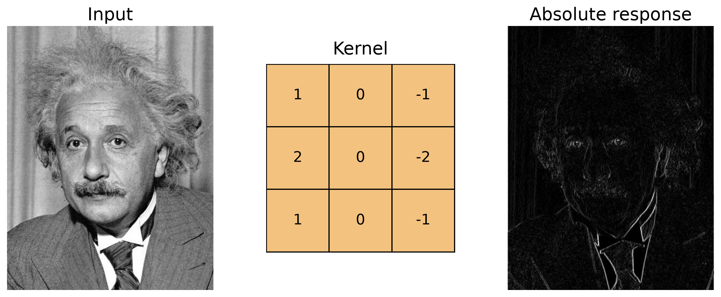
The absolute value displays both dark-to-light and light-to-dark transitions as bright edges.
Practice:
Examine the kernel and predict which image structures will produce the strongest response.
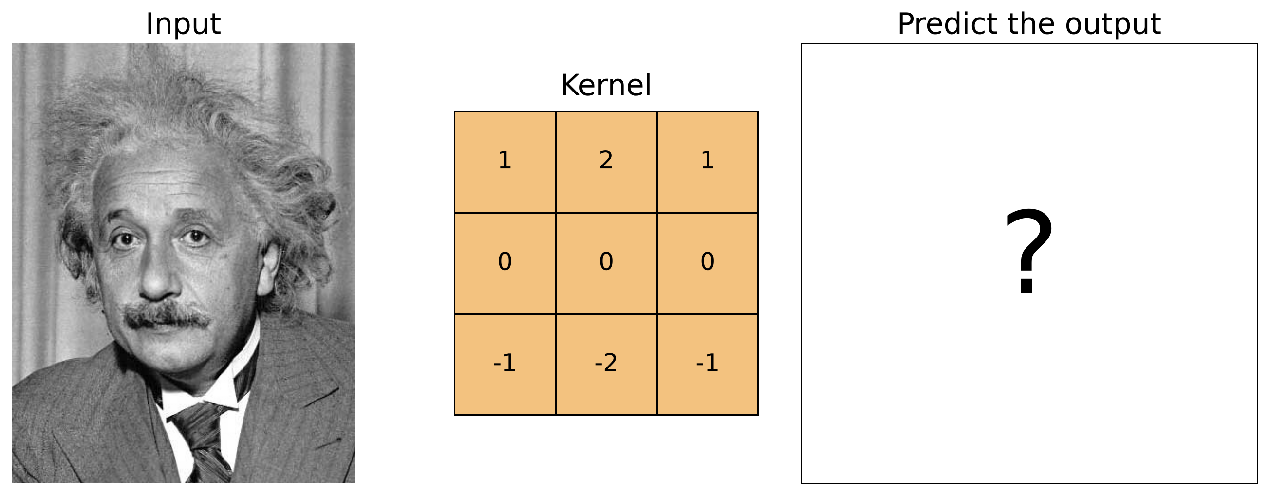
- Will the kernel respond to horizontal or vertical edges?
- Which regions of the image will have a response near zero?
Sobel \(y\): Detecting Horizontal Edges
This kernel responds strongly to horizontal edges.
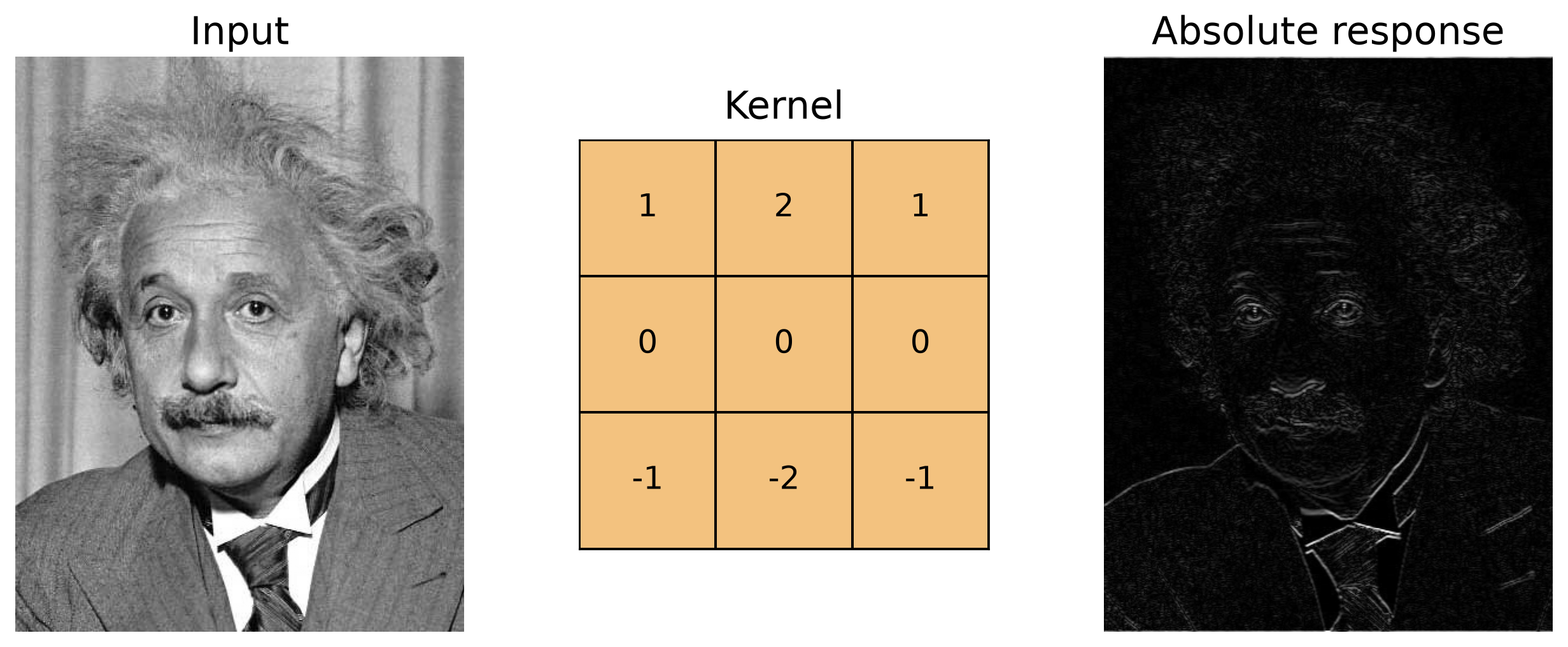
The sign of the original response indicates the direction of the intensity transition.
Practice: Subtracting the Local Average
What remains after subtracting the local \(3\times3\) average from the center pixel?
\[ h_{\text{detail}} = \delta-h_{\text{box}}. \]
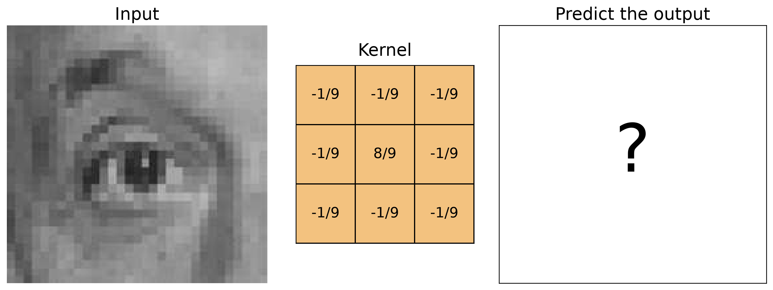
Local-Detail Kernel Extracts High Frequencies
The kernel removes smooth content and preserves rapid intensity changes:
\[ y = I-\operatorname{boxblur}(I). \]
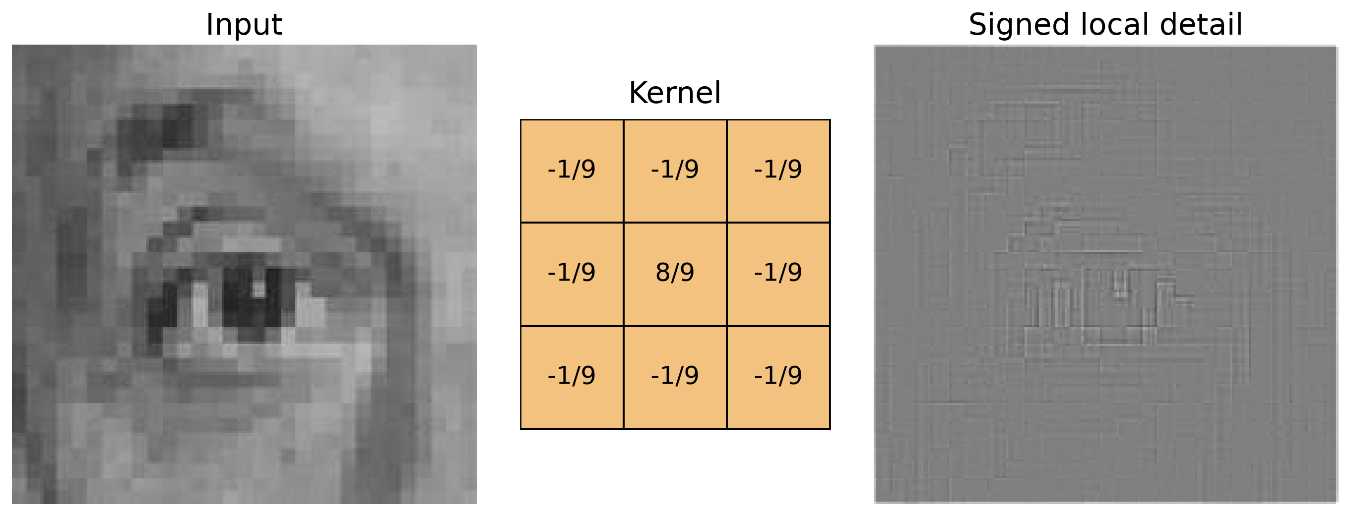
Mid-gray represents weak response; brighter or darker values represent strong filter response.
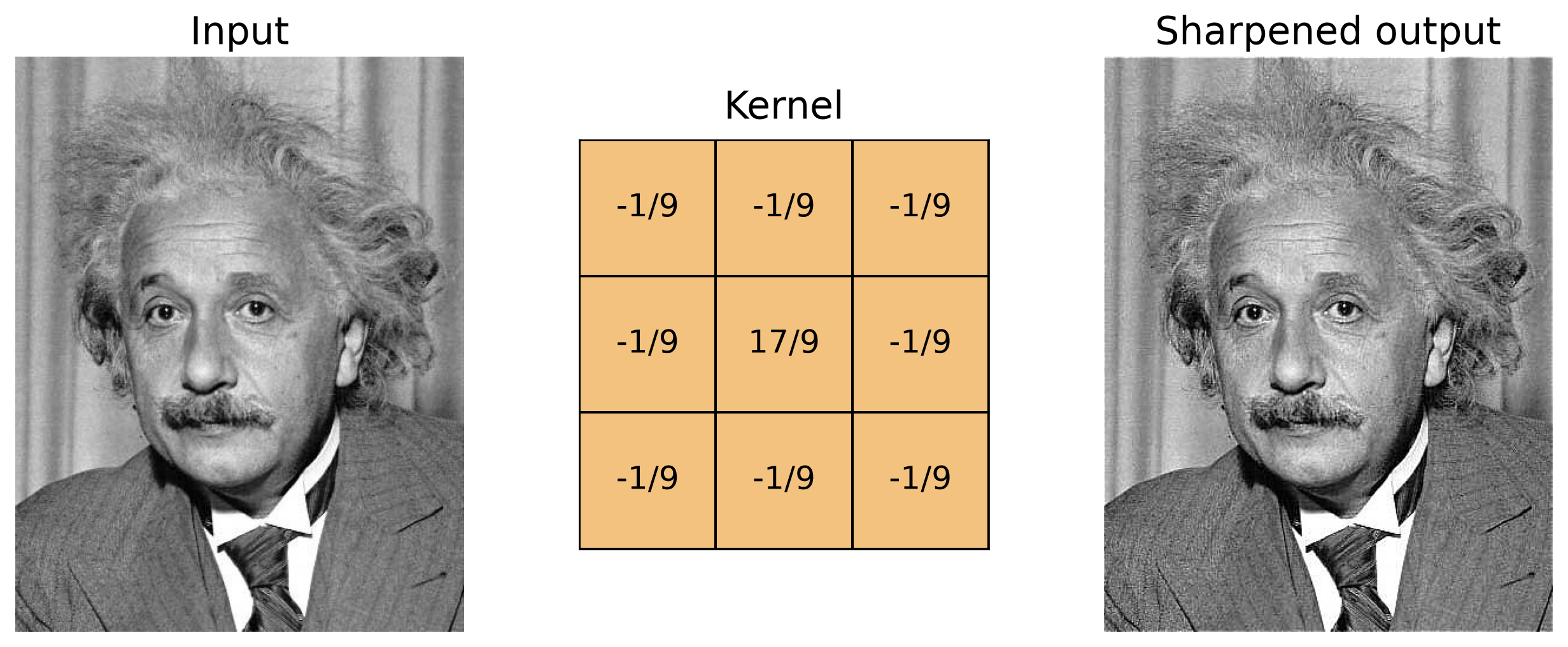
Adding Local Detail Sharpens the Image
Sharpening adds the extracted high-frequency detail back to the original image:
\[ h_{\text{sharp}} = \delta+\left(\delta-h_{\text{box}}\right) \] \[ y = I+\left(I-\operatorname{boxblur}(I)\right) \]
Filter Responses Can Be Negative
- Consider the horizontal-edge Sobel kernel \(h\).
- A Sobel filter estimates an image derivative, so output is not restricted to the range \([0,255]\) or \([0, 1]\).
- Positive and negative values represent opposite edge polarities.
- Values near zero indicate little intensity change.
\[ h= \begin{bmatrix} 1&2&1\\ 0&0&0\\ -1&-2&-1 \end{bmatrix} \]
img = cv2.imread("assets/03_filtering/red-rock.jpg", cv2.IMREAD_GRAYSCALE)
h_y = np.array([[1, 2, 1],
                [0, 0, 0],
                [-1, -2, -1]], dtype=np.float32)
img_out = cv2.filter2D(img, cv2.CV_32F, h_y, borderType=cv2.BORDER_CONSTANT)
limit = np.abs(img_out).max()

fig, ax = plt.subplots(1, 2, figsize=(6.5, 4))
ax[0].imshow(img, cmap="gray"); ax[0].set_title("Input")
ax[1].imshow(img_out, cmap="gray", vmin=-limit, vmax=limit)
ax[1].set_title("Signed filter response")
for a in ax: a.axis("off")
plt.tight_layout(); plt.show()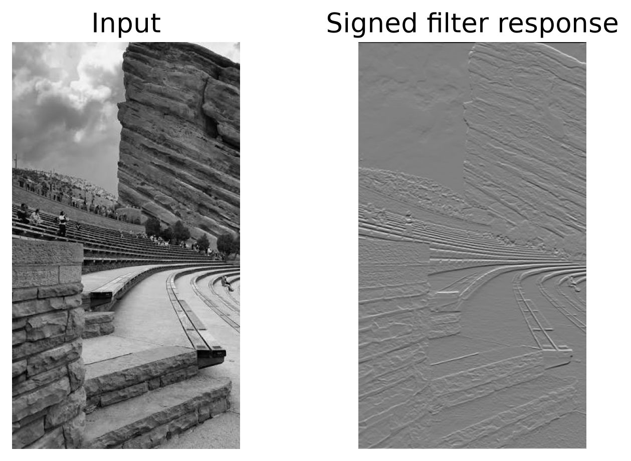
Visualizing Signed Filter Responses
The signed filter response can be transformed differently depending on what we want to visualize.
- In the signed response, zero is centered at gray.
- Clipping negative values removes one edge polarity.
- The absolute response shows edge strength but discards polarity.
limit = max(float(np.abs(img_out).max()), 1)

images = [img_out, np.clip(img_out, 0, None), np.abs(img_out)]

titles = ["Signed", "Neg clipped", "Absolute val"]
fig, ax = plt.subplots(1, 3, figsize=(6.5, 4))
for a, image, title in zip(ax, images, titles):
    signed = title == "Signed"
    a.imshow(image, cmap="gray", vmin=-limit if signed else 0, vmax=limit)
    a.set_title(title); a.axis("off")
plt.tight_layout(); plt.show()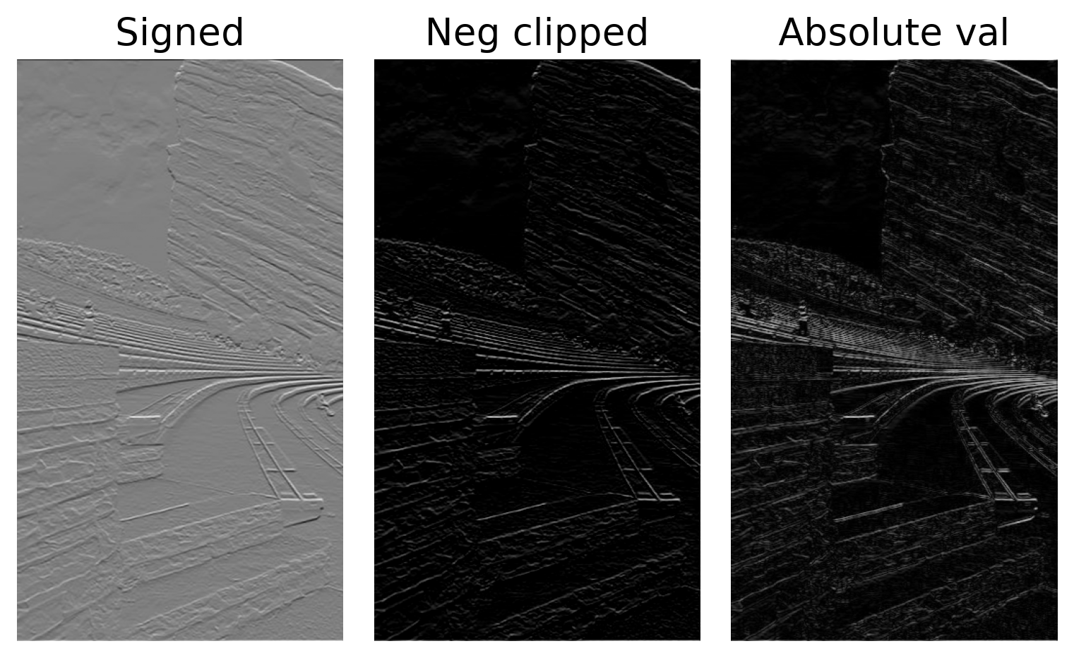
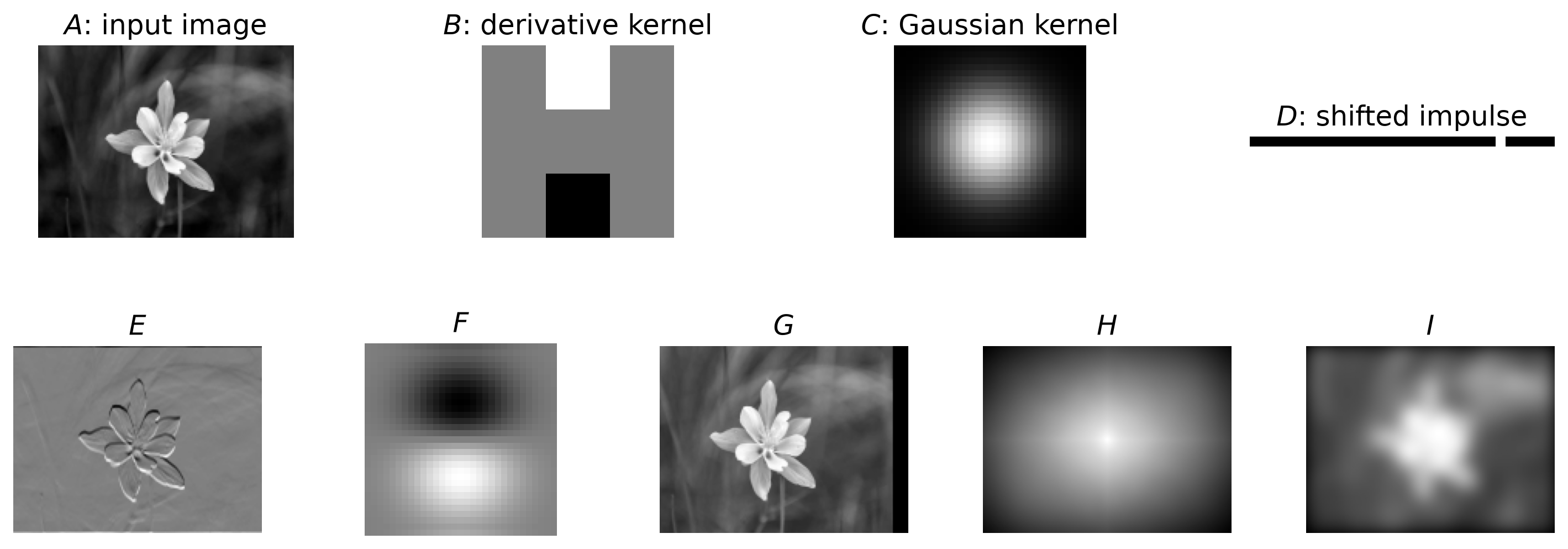
Practice: Match Each Filter to Its Output
Select E, F, G, H, or I for each filter. One candidate is not used.
\[ 1.\;A*B=? \qquad 2.\;B*C=? \qquad 3.\;A*D=? \qquad 4.\;A*A=? \]
Practice: Answers
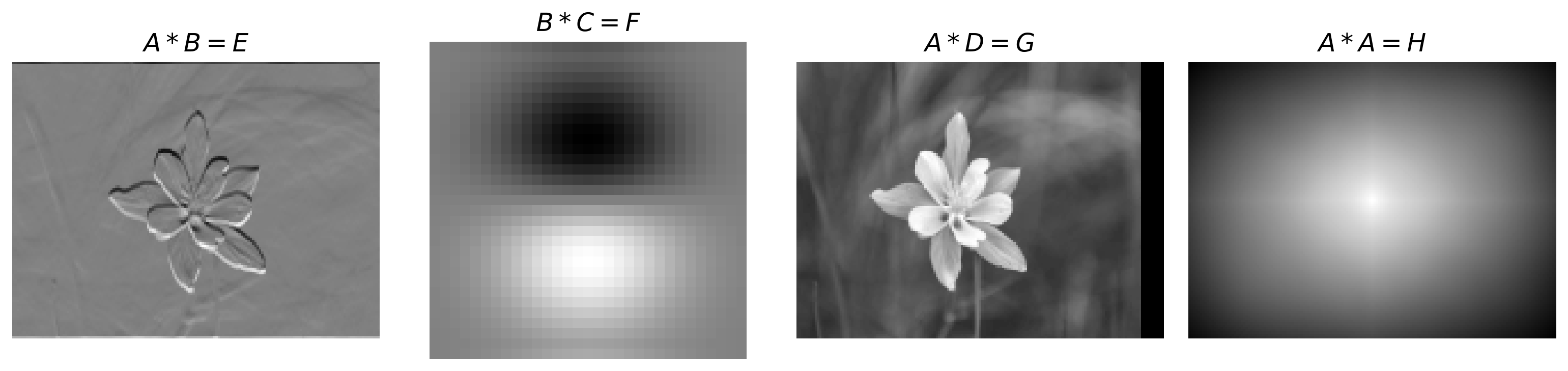
- \(A*B=E\): the derivative kernel produces an edge response.
- \(B*C=F\): smoothing the derivative kernel produces a derivative-of-Gaussian kernel.
- \(A*D=G\): correlation with the shifted impulse shifts the image.
- \(A*A=H\): correlation the image with itself produces a broad self-correlation response.
The unused candidate is \(I=A*C\), the Gaussian-smoothed image.
Correlation as Template Matching
- Use an image patch as the filter kernel and correlate it across the image: \[ y[m,n]=\sum_k\sum_l h[k,l]\,I[m+k,n+l] \]
- The largest response is the location that best matches the template.
import cv2

path = "assets/03_filtering/colorado-flowers.jpg"
box = (60, 65, 125, 135) # x0, y0, width, height

I = cv2.imread(path, cv2.IMREAD_GRAYSCALE).astype(np.float32)/255
x0, y0, w, ht = box
h = I[y0:y0+ht, x0:x0+w]

y = cv2.filter2D(I, cv2.CV_32F, h, borderType=cv2.BORDER_CONSTANT)
_, score, _, (px,py) = cv2.minMaxLoc(y)

selected = I.copy(); cv2.rectangle(selected,(x0,y0),(x0+w,y0+ht),1,3)
match = I.copy()
cv2.rectangle(match,(px-w//2,py-ht//2),(px+w//2,py+ht//2),1,3)

fig, ax = plt.subplots(2,2,figsize=(6.5,4))
ims = [selected,h,y,match]
titles = ["Selected template","Template $h$","Correlation output $y$","Largest response"]

for a, im, title in zip(ax.flat,ims,titles):
    a.imshow(im,cmap="gray"); a.set_title(title); a.axis("off")

plt.tight_layout(pad=.3); plt.show()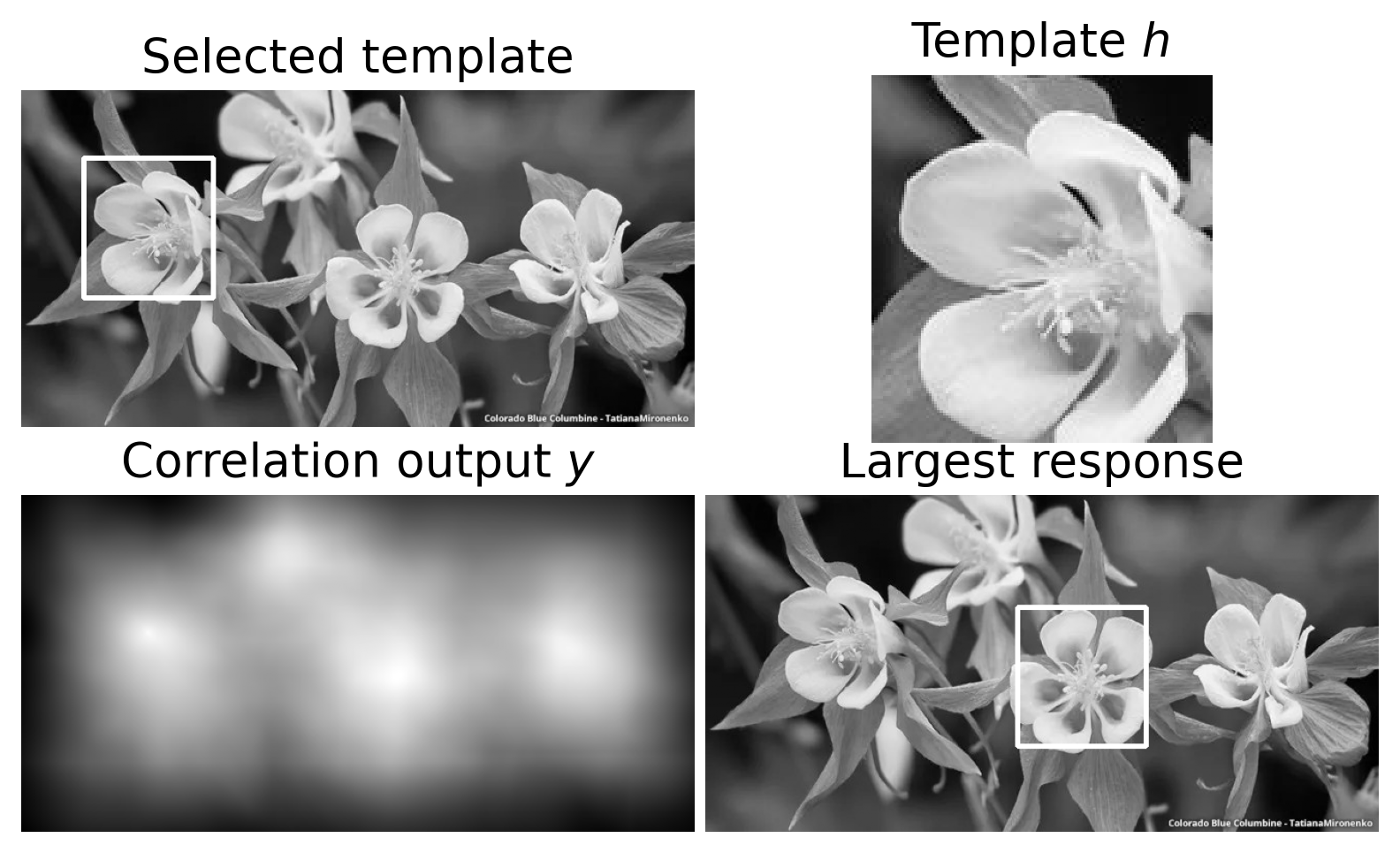
Brightness Can Dominate Correlation
- Raw correlation computes a dot product, so brighter regions can produce larger responses.
- Subtract the template mean: \(f_0 = f-\bar f\)
- Now positive and negative values describe the pattern relative to its local brightness.
h0 = h - h.mean()
y = cv2.filter2D(I, cv2.CV_32F, h0, borderType=cv2.BORDER_CONSTANT)

_, score, _, (px,py) = cv2.minMaxLoc(y)
match = I.copy()
cv2.rectangle(match,(px-w//2,py-ht//2),(px+w//2,py+ht//2),1,3)

fig, ax = plt.subplots(2,2,figsize=(6.5,4.5))
ax[0,0].imshow(h0,cmap="gray"); ax[0,0].set_title("Zero-mean $h$")
ax[1,0].imshow(y,cmap="gray"); ax[1,0].plot(px,py,"r.",ms=8)
ax[1,0].set_title("Correlation output $y$")
ax[1,1].imshow(match,cmap="gray"); ax[1,1].set_title(f"Peak: ({px}, {py})")
for a in ax.flat: a.axis("off")
plt.tight_layout(pad=.3); plt.show()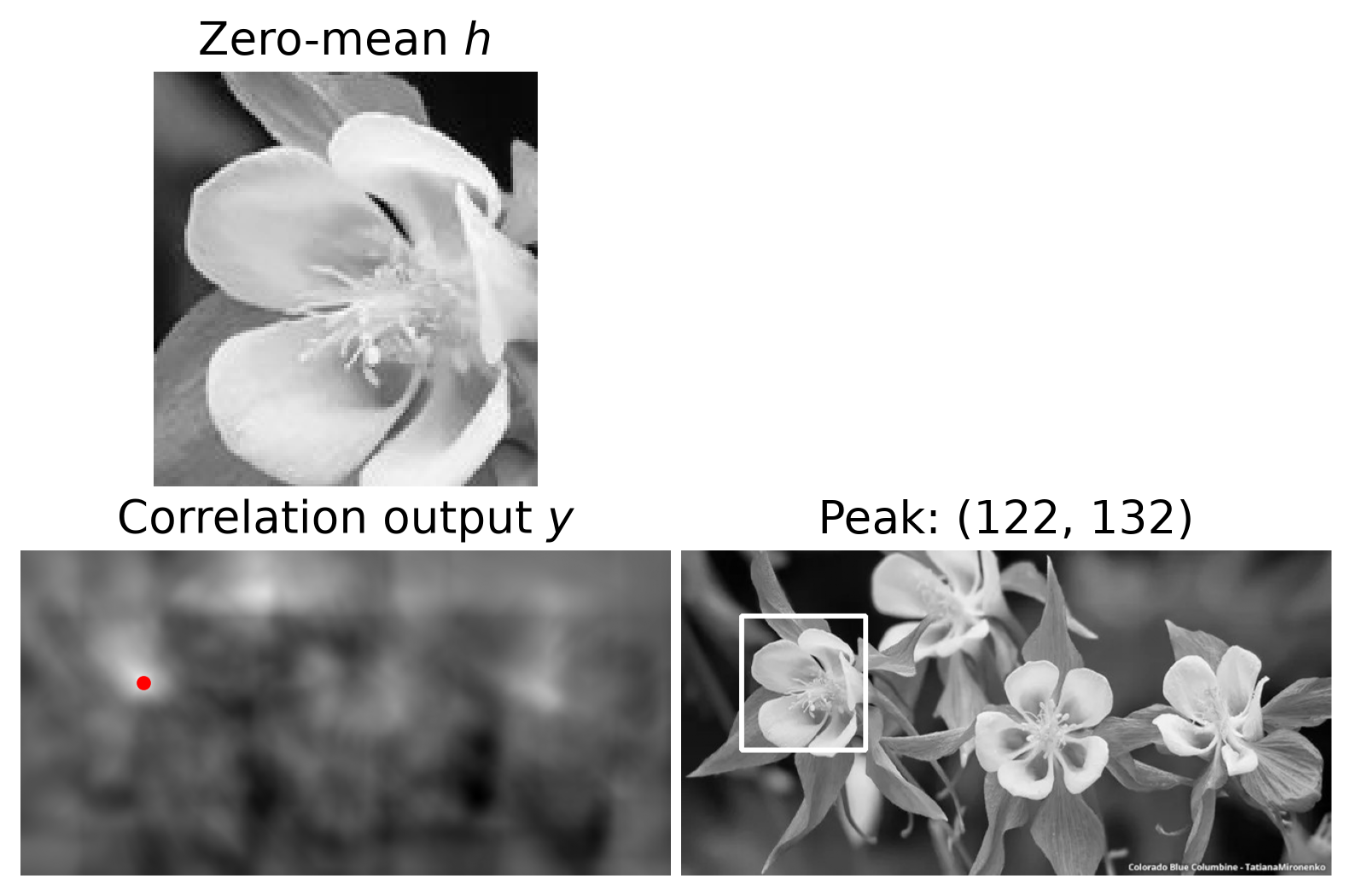
Use Correlation, Not Convolution, for Template Matching
- Correlation compares the template in its original orientation.
- Convolution compares against a template rotated by \(180^\circ\).
- For template matching, use correlation so the template orientation is preserved.
kernels = [h0, cv2.flip(h0,-1)]
names = ["Correlation","Convolution"]

fig, ax = plt.subplots(2,2,figsize=(6.5,4.4))

for r, (hk,name) in enumerate(zip(kernels,names)):
    y = cv2.filter2D(I, cv2.CV_32F, hk, borderType=cv2.BORDER_CONSTANT)
    _, score, _, (px,py) = cv2.minMaxLoc(y)

    match = I.copy()
    cv2.rectangle(match,(px-w//2,py-ht//2),(px+w//2,py+ht//2),1,3)

    ax[r,0].imshow(hk,cmap="gray")
    ax[r,1].imshow(match,cmap="gray")
    ax[r,0].set_title(f"{name} kernel")
    ax[r,1].set_title(f"Peak response = {score:.1f}")

for a in ax.flat: a.axis("off")
plt.tight_layout(pad=.3); plt.show()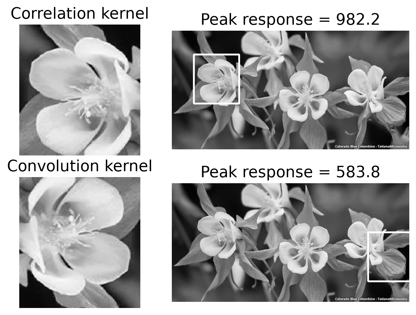
Median Filter
- A median filter is a nonlinear rank filter: \[ y[m,n]=\operatorname{median}\{I[m+k,n+l]\}_{(k,l)\in\Omega}. \]
- It replaces the center pixel by the middle value in the local neighborhood.
- Unlike a linear filter, there is no kernel \(h[k,l]\) such that \(y[m,n]=\sum_k\sum_l h[k,l]\,I[m+k,n+l].\)
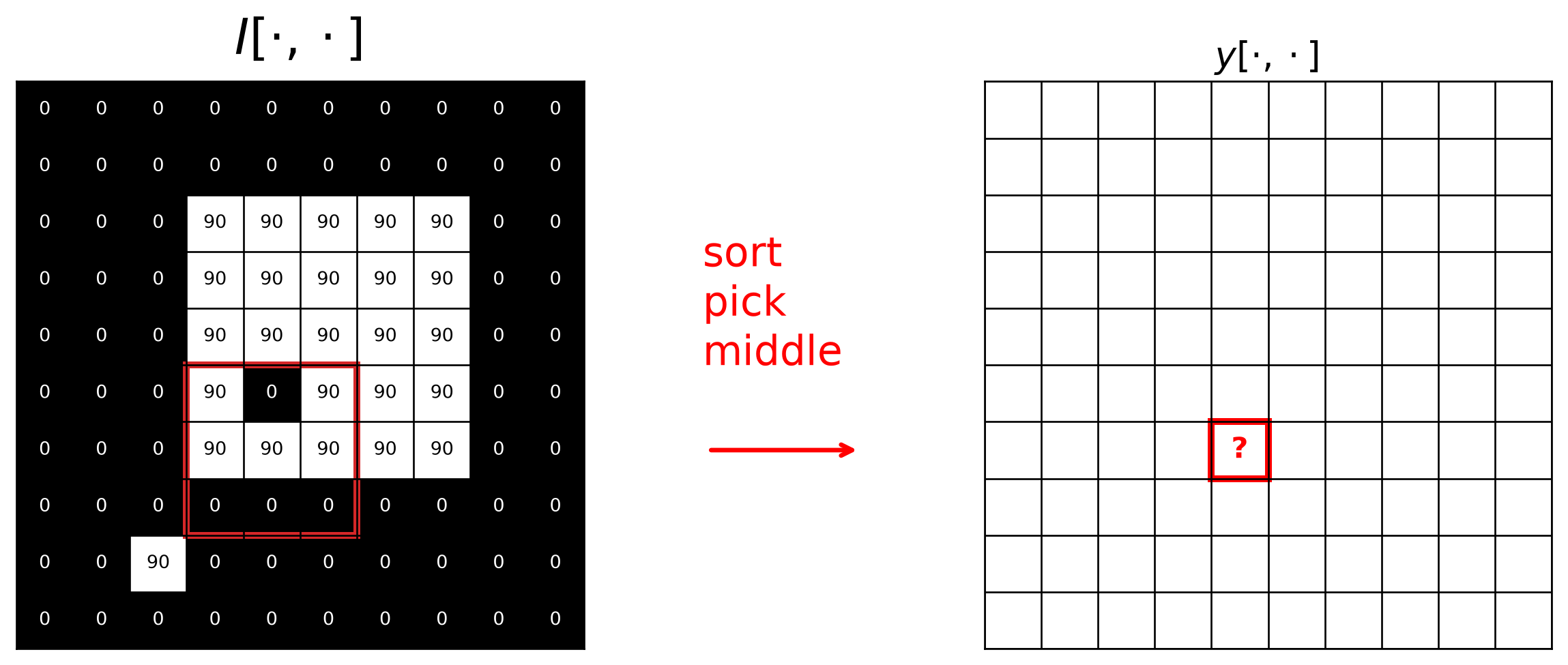
Salt-and-Pepper Noise: Mean vs. Median
Impulse noise replaces some pixels with 0 or 255.
A mean filter averages these outliers with their neighbors, while a median filter can reject them.
path = "assets/03_filtering/colorado-flower.jpg"
I0 = cv2.imread(path, cv2.IMREAD_GRAYSCALE)
I0 = cv2.resize(I0, (380,255))

# Add salt-and-pepper noise
rng, p = np.random.default_rng(7), 0.03
Isp = I0.copy(); M = rng.random(I0.shape)
Isp[M < p] = 0; Isp[M > 1-p] = 255

# Compare mean and median filtering
Imean3 = cv2.blur(Isp, (3,3), borderType=cv2.BORDER_REFLECT)
Imed3  = cv2.medianBlur(Isp, 3)

fig, ax = plt.subplots(2,2,figsize=(6.5,4.4))
for a, im, t in zip(ax.flat,
    [I0, Isp, Imean3, Imed3],
    ["Original $I$", "Salt-and-pepper noise", "3×3 mean", "3×3 median"]):
    panel(a, im, t)
plt.tight_layout(pad=.3); plt.show()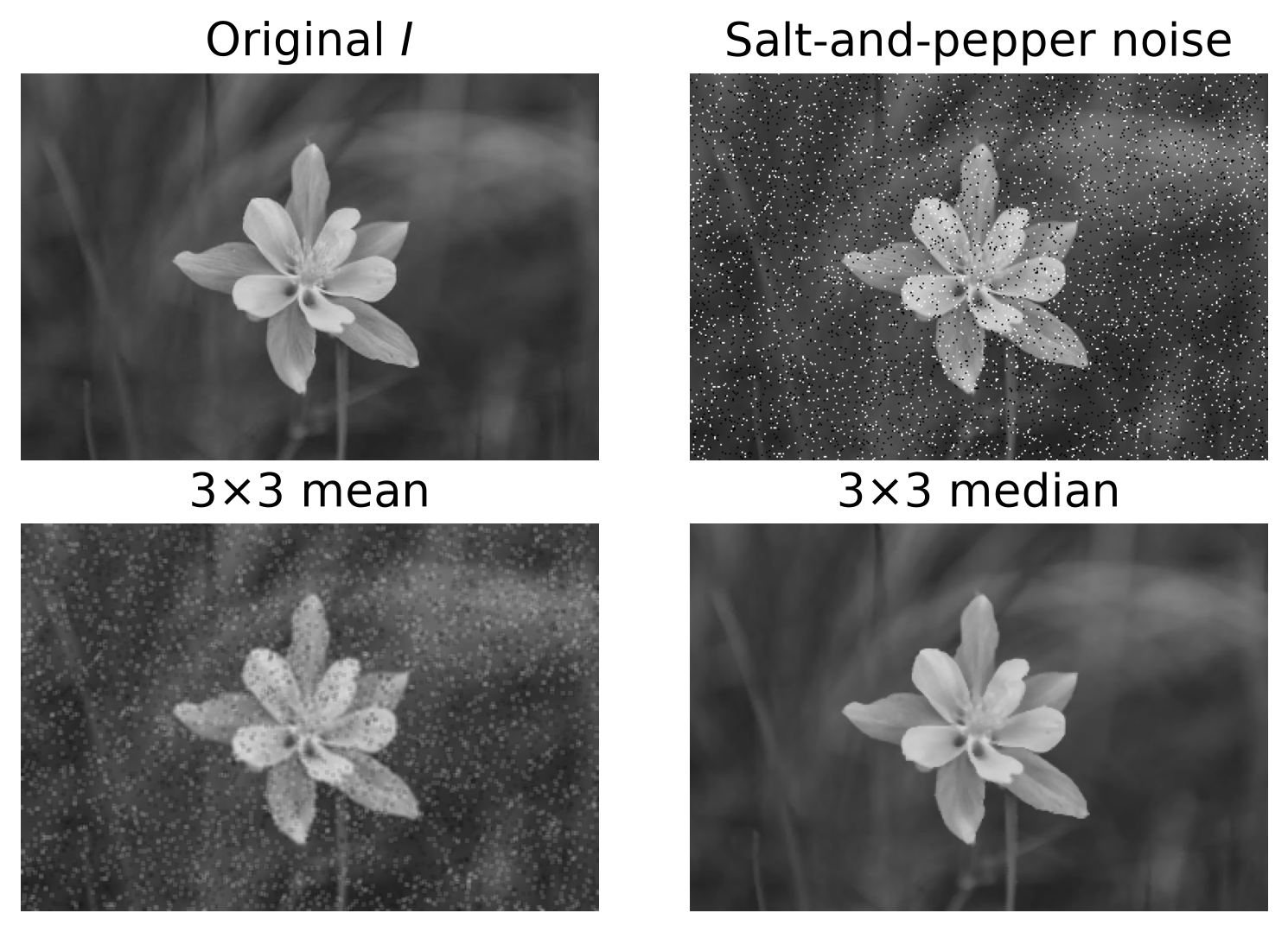
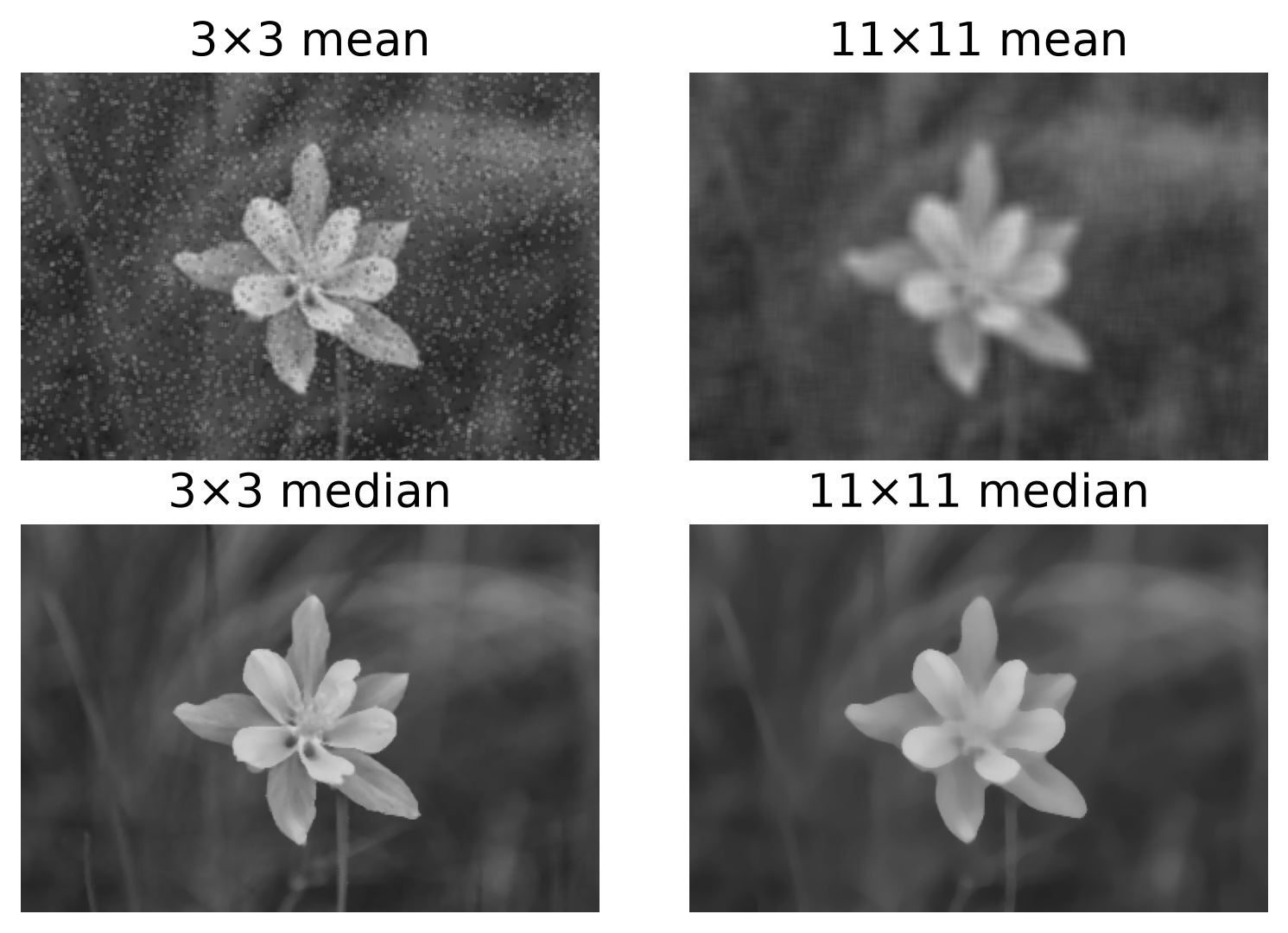
Window Size Matters
- Larger windows remove more noise, but they also remove more image detail.
# Mean filters
Imean3  = cv2.blur(Isp, (3,3),   borderType=cv2.BORDER_REFLECT)
Imean11 = cv2.blur(Isp, (11,11), borderType=cv2.BORDER_REFLECT)

# Median filters
Imed3  = cv2.medianBlur(Isp, 3)
Imed11 = cv2.medianBlur(Isp, 11)

fig, ax = plt.subplots(2,2,figsize=(6.5,4.4))
for a, im, t in zip(ax.flat,
    [Imean3, Imean11, Imed3, Imed11],
    ["3×3 mean", "11×11 mean", "3×3 median", "11×11 median"]):
    panel(a, im, t)
plt.tight_layout(pad=.3); plt.show()