Lecture 05 — Fourier Transform
Lecture 5
Fourier Transform
Fourier’s Idea
Can we build a complicated signal from simple waves?
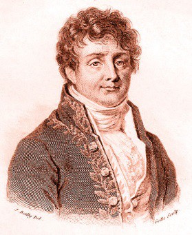 Joseph Fourier (1768–1830)
The Fourier series claim (1807):
Any univariate function can be rewritten as a weighted sum of sines and cosines of different frequencies.
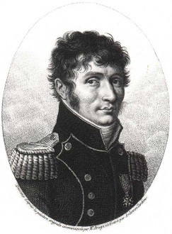 Malus
Malus
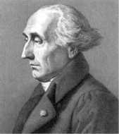 Lagrange
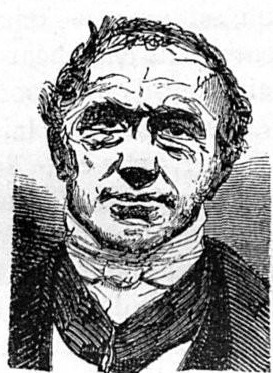 Legendre
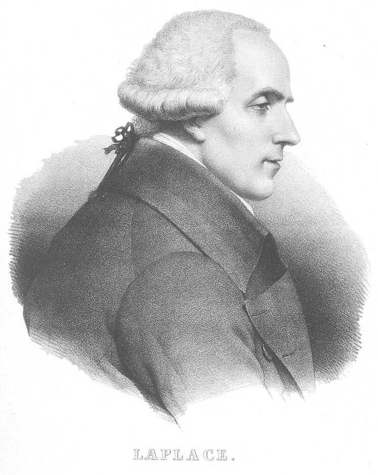 Laplace
The initial reviewers (Lagrange, Laplace, Monge, and Lacroix) were skeptical, partly because the proofs lacked rigor. Publication of his work was initially withheld.
The later committee, which included Lagrange, Laplace, Malus, and Legendre, awarded Fourier a prize but criticized the generality and rigor of his analysis.
Is Fourier’s Claim True?
Well, almost.
The theorem requires additional conditions:
- A sufficient condition is that the function is periodic and piecewise smooth.
- At continuous points, the series converges to the function’s value.
- At a jump, it converges to the average of the values on either side.
Very surprising result at the time, because it implied that
- Even signals with sharp corners or jumps can have a representation built from smooth sine and cosine waves.
Joseph Fourier
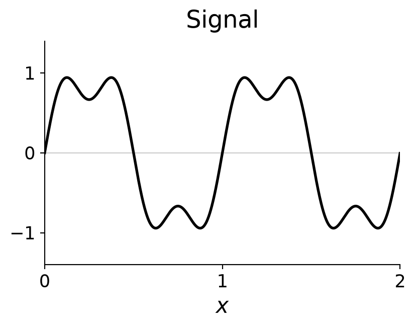
Example: Adding Sinusoids
How would you generate this function?
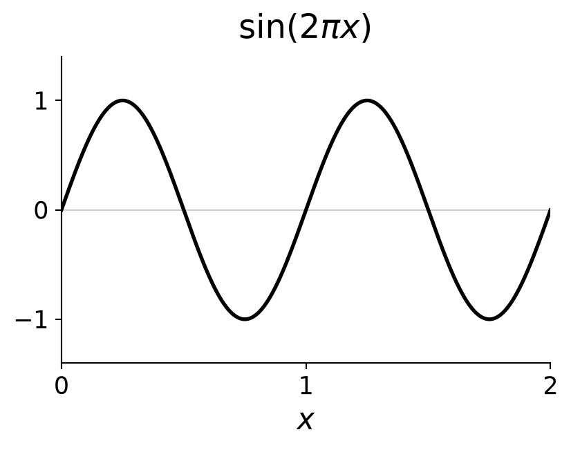
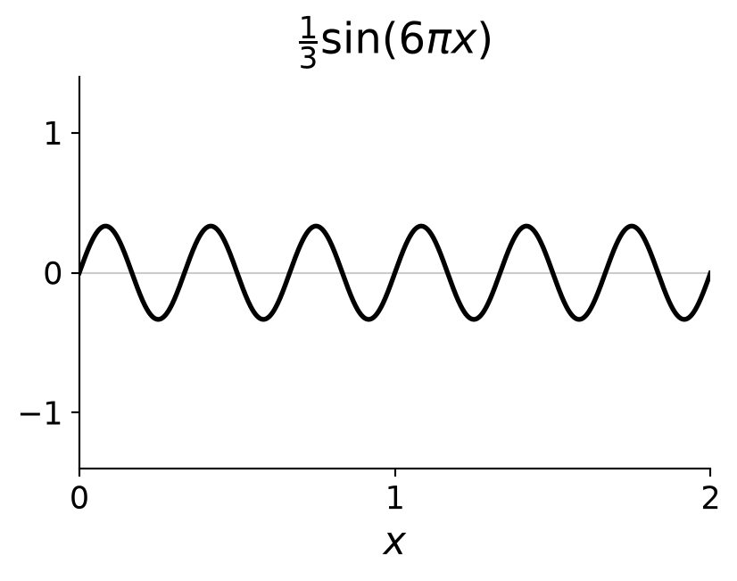
\[ y(x) = \sin(2\pi x) + \frac{1}{3}\sin(6\pi x) \]
Example: Approximating a Square Wave
How would you generate this function?
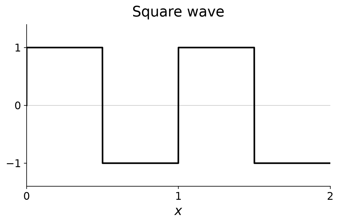
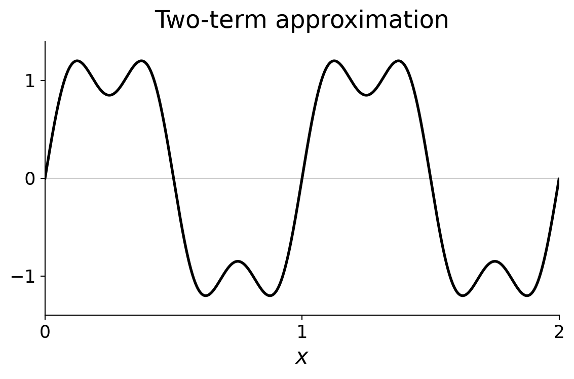
\[ \frac{4}{\pi} \left[ \sin(2\pi x) + \frac{1}{3}\sin(6\pi x) \right] \]
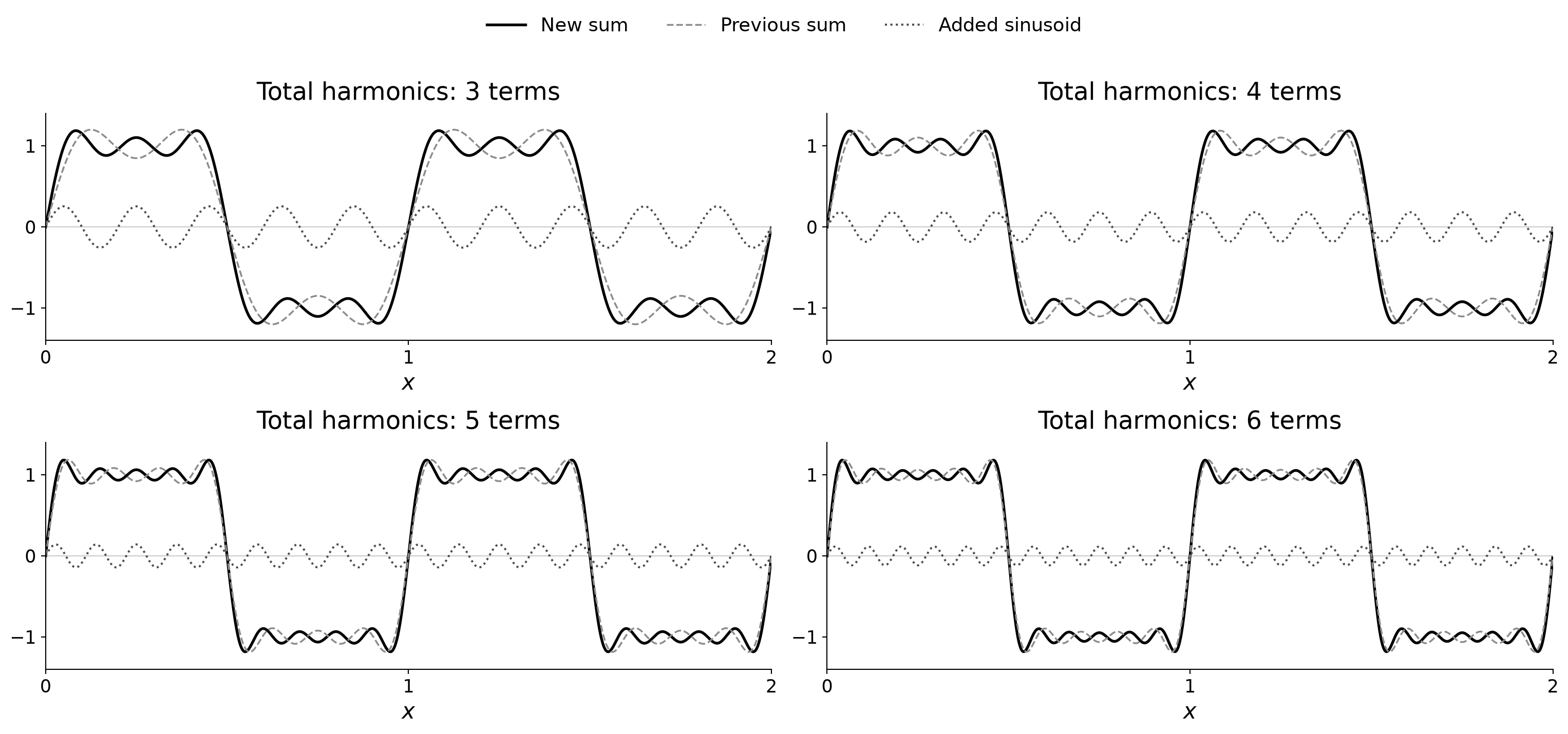
What happens if we add higher-frequency sinusoids?
Adding More Harmonics
Add the next harmonic at each step:
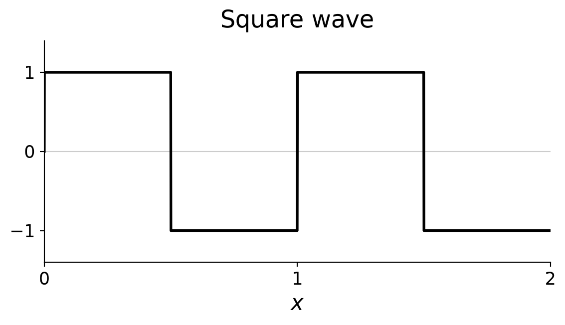
The Square-Wave Fourier Series
How would you express this mathematically?
General Fourier series:
\[ y(x) = c_0 + \sum_{k=1}^{\infty} A_k \sin(2\pi k f_0 x + \phi_k) \]
For this square wave, \(c_0=0\) and \(f_0=1\):
\[ y(x) = \sum_{\substack{k=1\\k\text{ odd}}}^{\infty} \frac{4}{k\pi}\sin(2\pi kx) \]
- Frequencies: \(1, 3, 5, 7, \ldots\)
- Amplitudes: \(\displaystyle \frac{4}{\pi}, \frac{4}{3\pi}, \frac{4}{5\pi}, \ldots\)
- Phases: \(0, 0, 0, \ldots\)
The Square Wave in the Frequency Domain
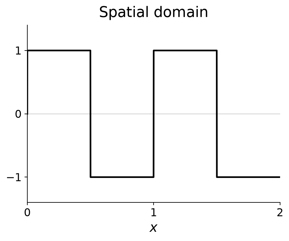
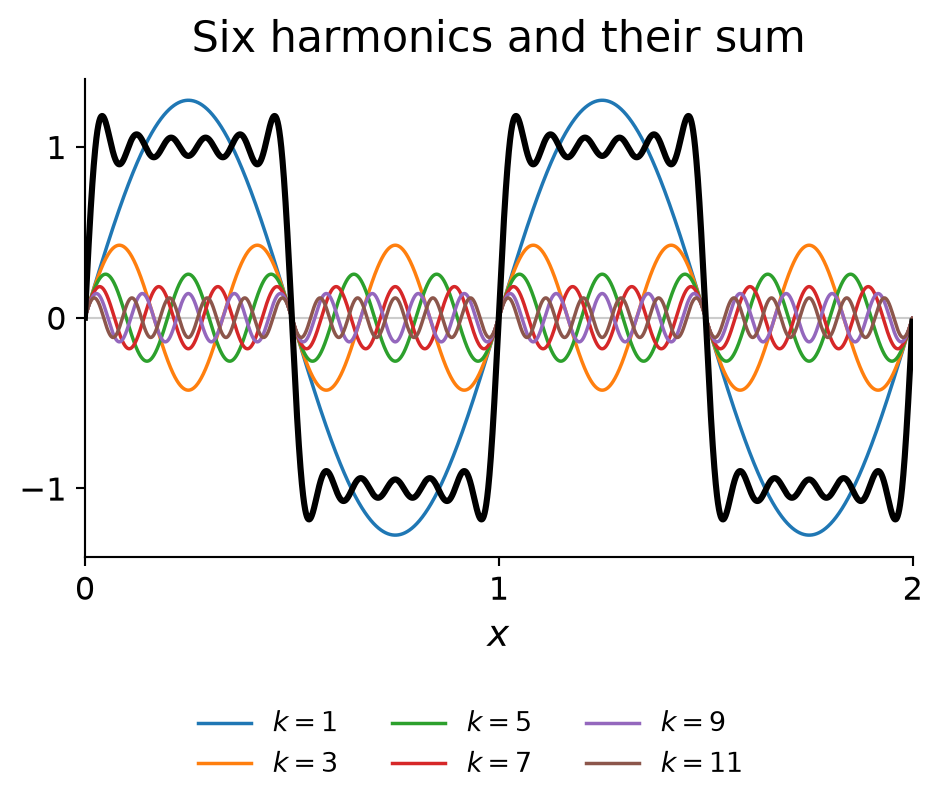
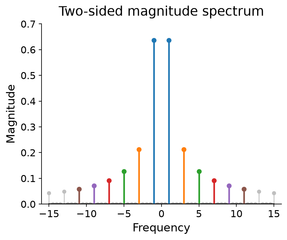
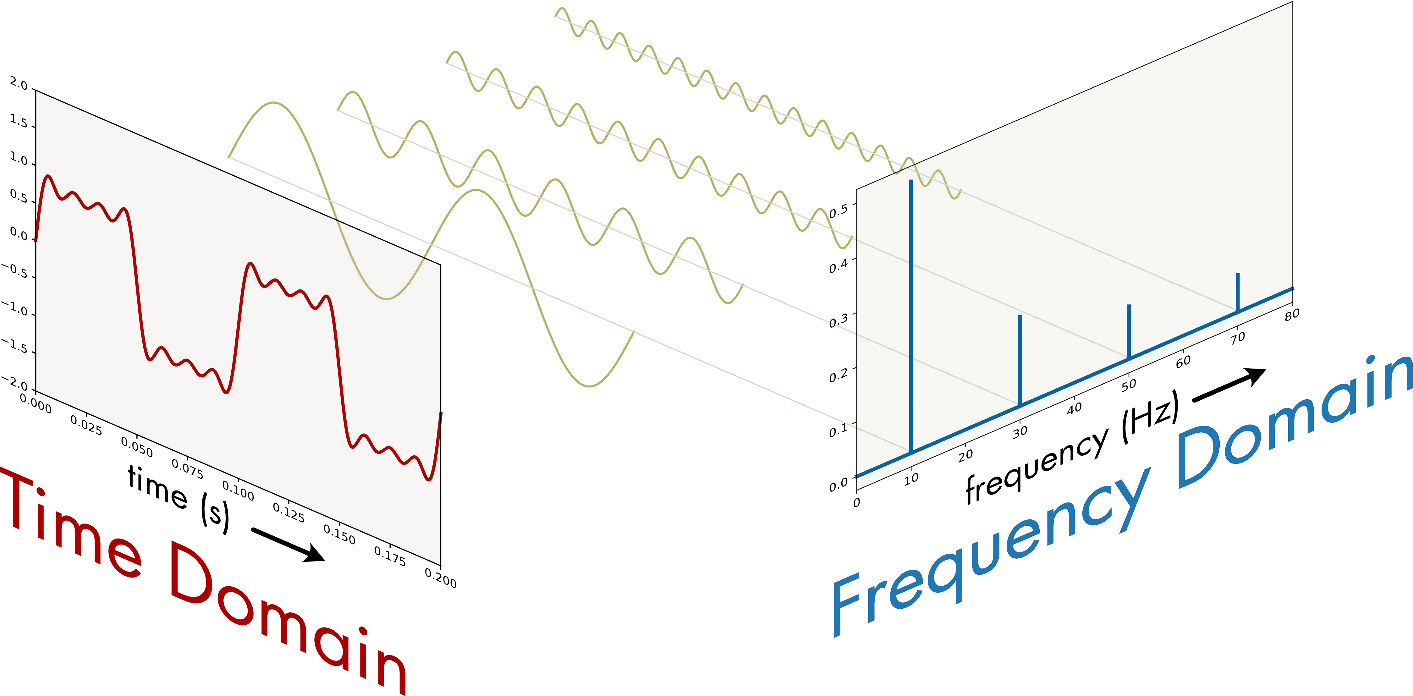
\[ y_6(x) = \frac{4}{\pi}\sin(2\pi x) + \frac{4}{3\pi}\sin(6\pi x) + \frac{4}{5\pi}\sin(10\pi x) + \frac{4}{7\pi}\sin(14\pi x) + \frac{4}{9\pi}\sin(18\pi x) + \frac{4}{11\pi}\sin(22\pi x) \]
Each sinusoid produces two peaks at frequencies \(\pm f\). Matching colors connect each sinusoid to its peaks.
The black curve in the middle shows the six-term sum; the ideal square wave requires infinitely many terms.
Visualizing the Frequency Spectrum
\[ f(x) = c_0 + \sin(2\pi x) + \frac{1}{3}\sin(6\pi x), \qquad c_0 = 1 \]
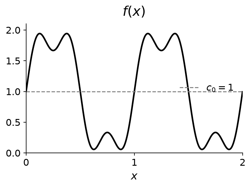
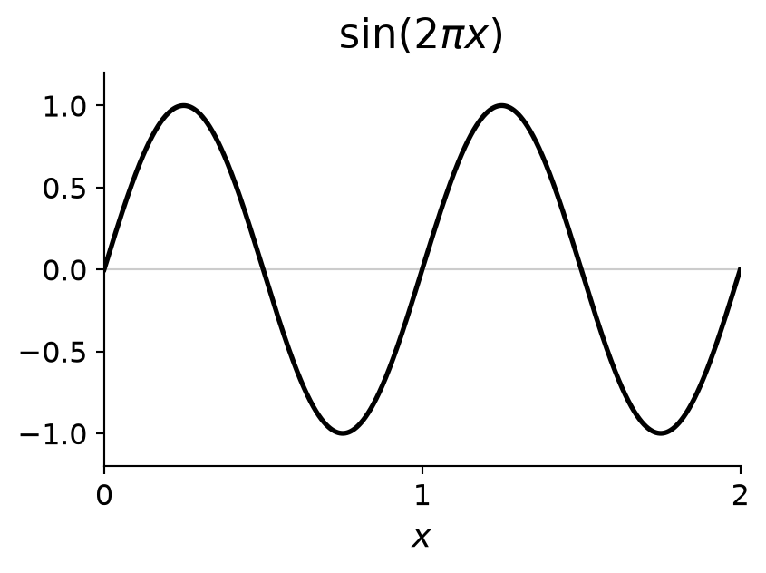
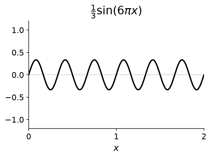
The constant \(c_0\) shifts the signal vertically without changing its oscillations.
How does each term appear in the frequency domain?
Visualizing the Frequency Spectrum
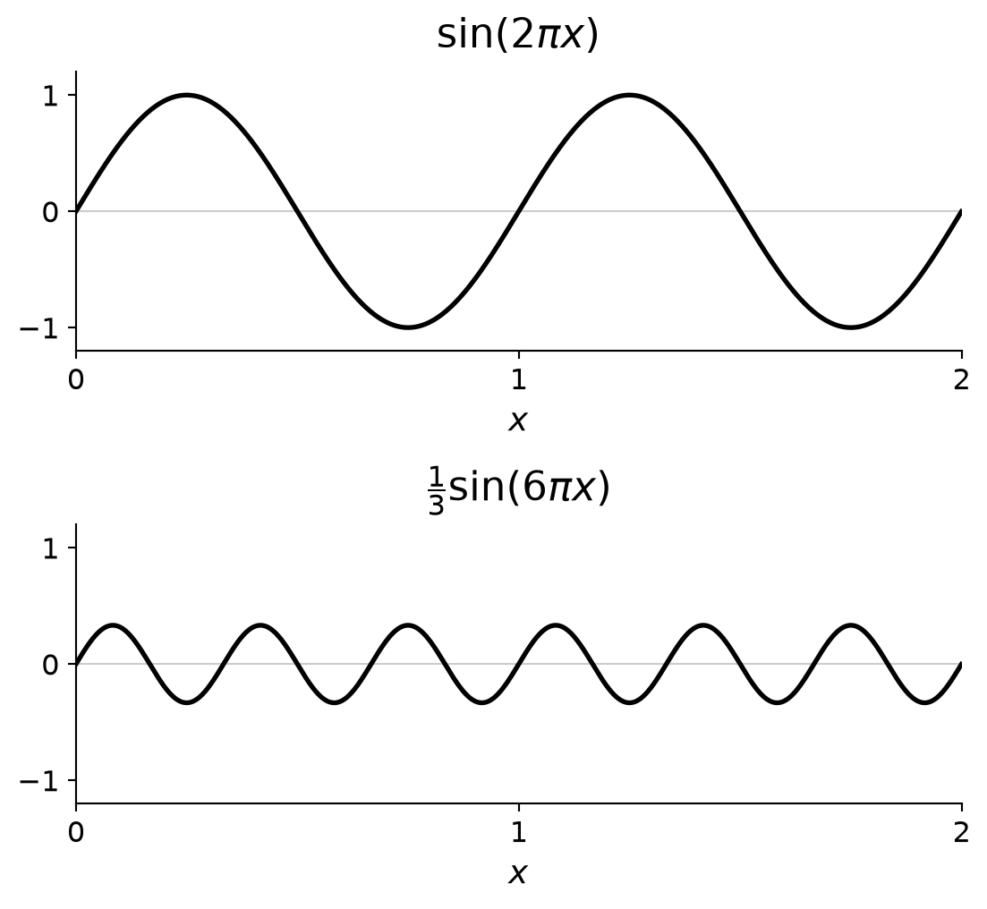
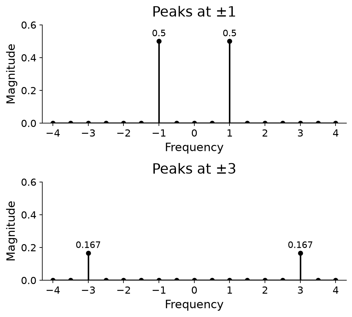
A sinusoid of amplitude \(A\) produces two peaks, each of height \(A/2\), at its positive and negative frequencies.
What Is at Zero Frequency?
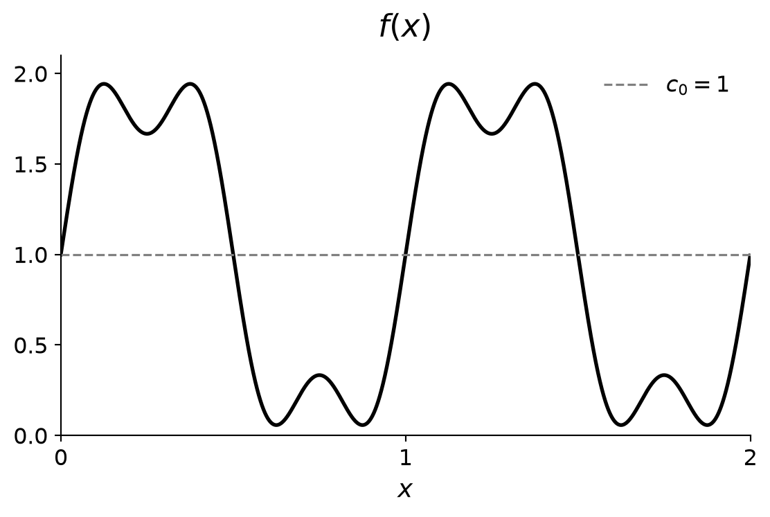
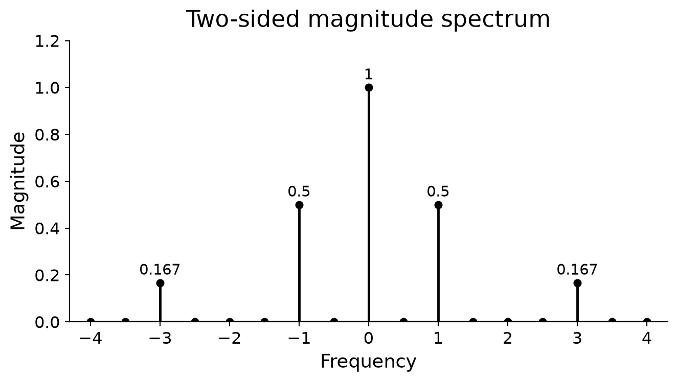
The DC component represents the signal’s mean value.
\[ c_0 = \frac{1}{N}\sum_{n=0}^{N-1} f(x_n) = 1 \]
The constant contributes one peak at zero frequency, with magnitude \(|c_0|\). It is not split into two peaks.
For images, the DC component corresponds to the average pixel intensity.
A 1D Signal as an Image
Repeat the same 1D intensity signal along every image row.
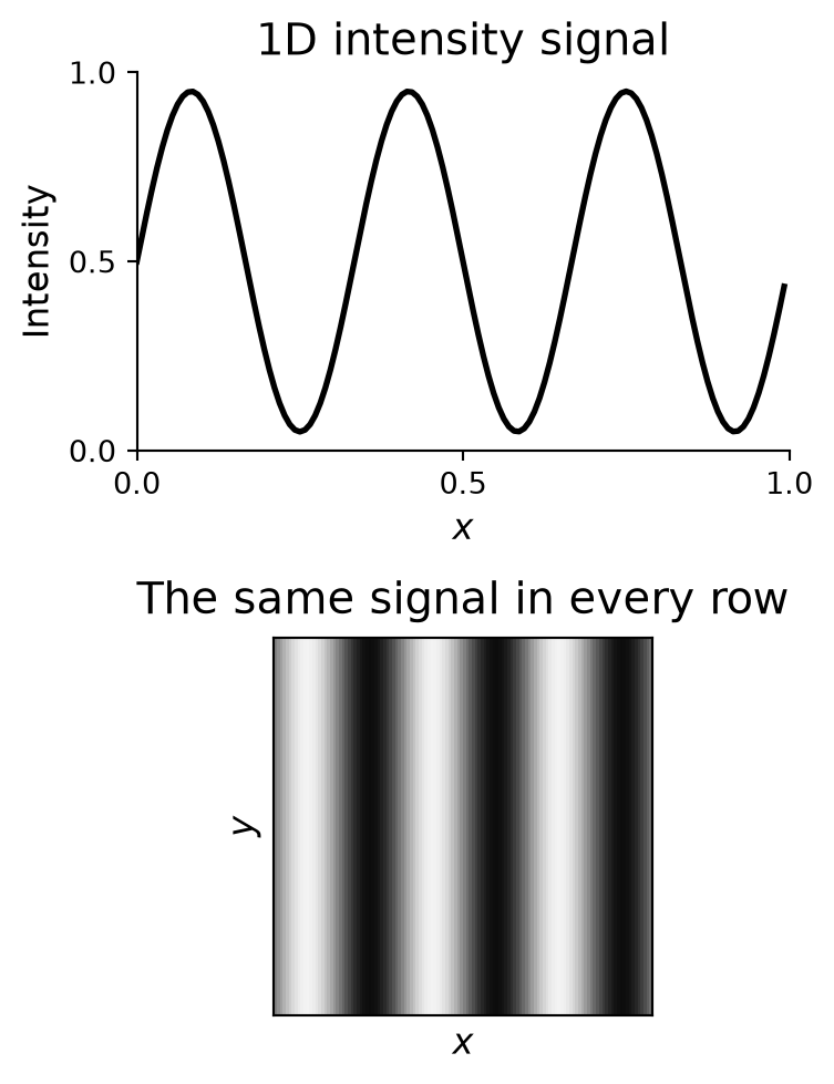
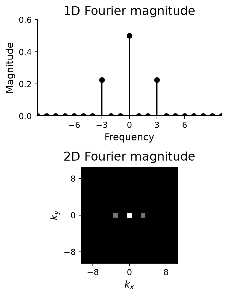
What do the three bright spots represent?
- Center: the mean image intensity.
- Side pair: the sinusoidal variation along \(x\). Every row is identical, so there is no variation along \(y\).
Stripe Spacing and Frequency
What changes when the stripes become narrower?
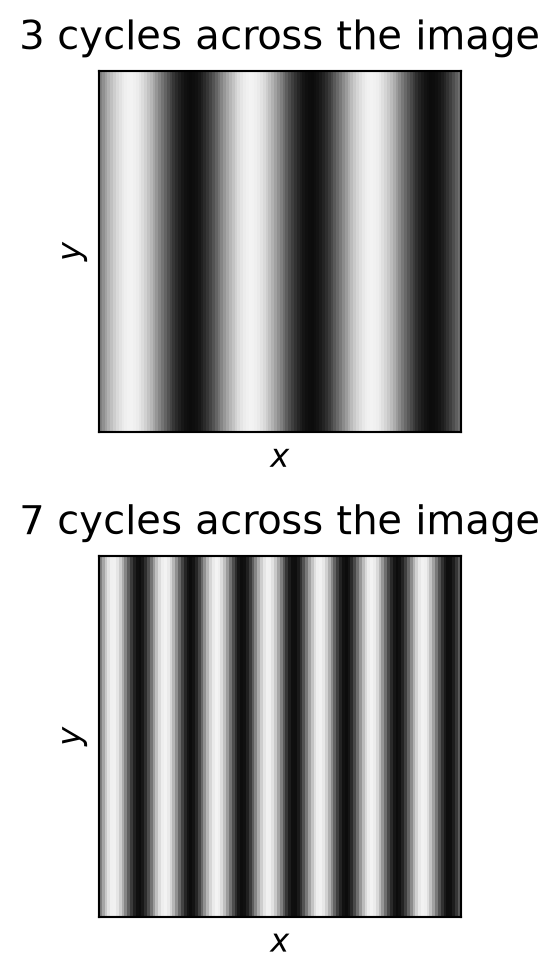
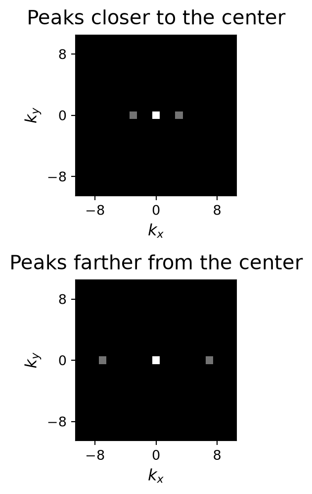
- Narrower stripes mean higher spatial frequency.
- The side peaks move farther from the center.
- The center spot stays the same because the mean intensity is unchanged.
Diagonal Stripes
Does the Fourier intensity change along \(x\), along \(y\), or both?
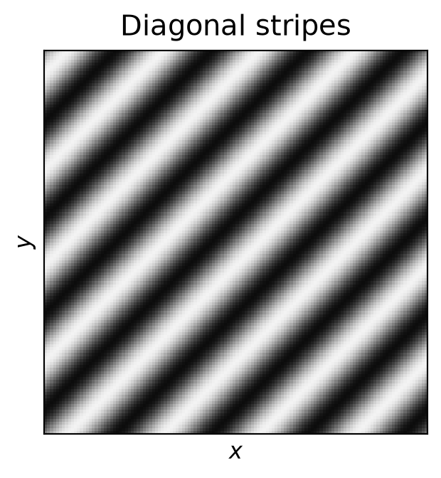
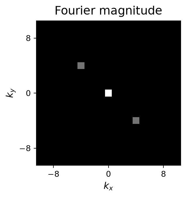
Both. The sinusoid varies along a diagonal direction.
- Its frequency has both horizontal and vertical components.
- The two side peaks lie off the horizontal and vertical axes.
- The line joining the two side peaks is perpendicular to the stripes.
Combining Patterns
What happens when we average these two images?
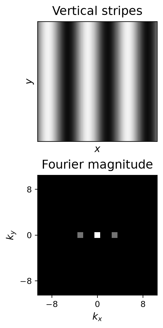
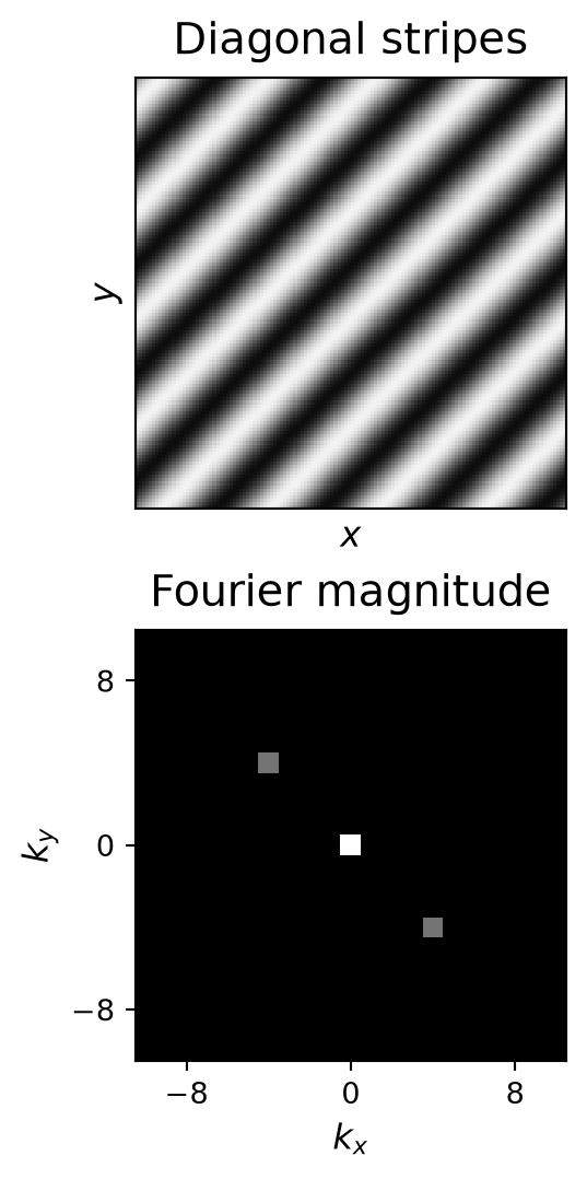
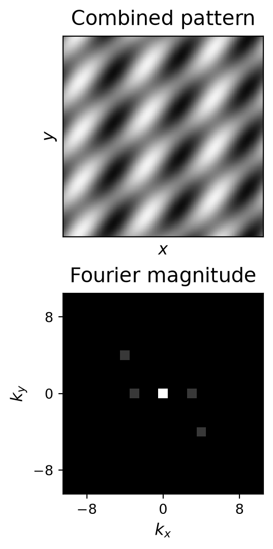
- Both peaks appear in the combined spectrum.
- Averaging halves each pattern’s contribution, so its side peaks become dimmer.
- The center spot stays the same because both images have the same mean intensity.
What About Nonperiodic Signals?
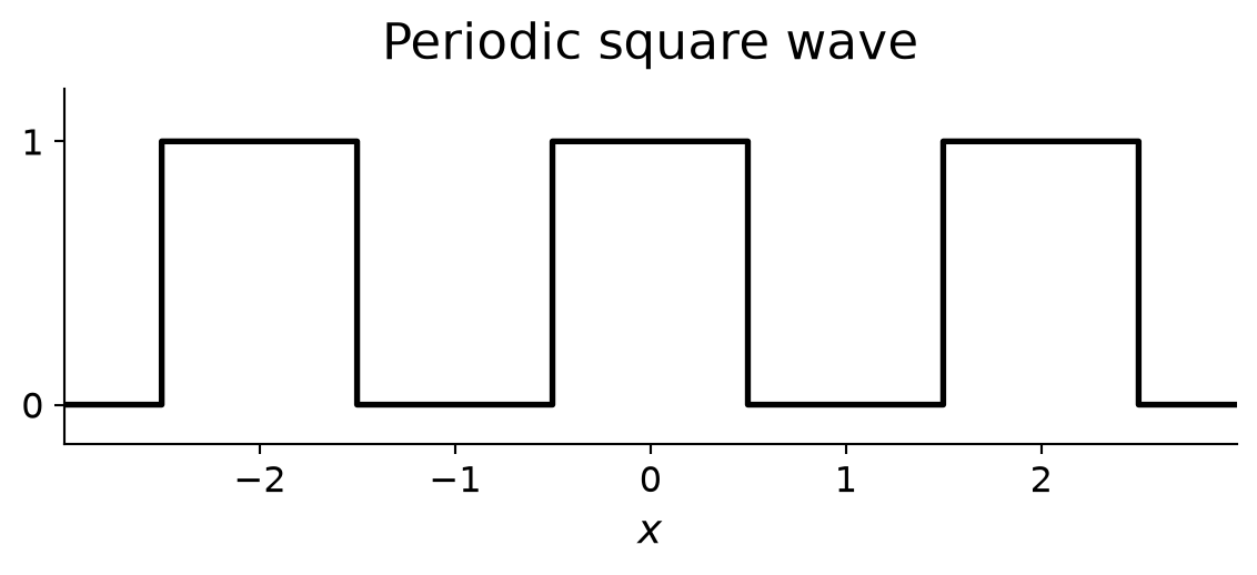
Fourier series represent periodic signals as sums of sinusoids.
Fourier series
- Signal pattern repeats with period \(T\).
- Uses a discrete set of frequencies.
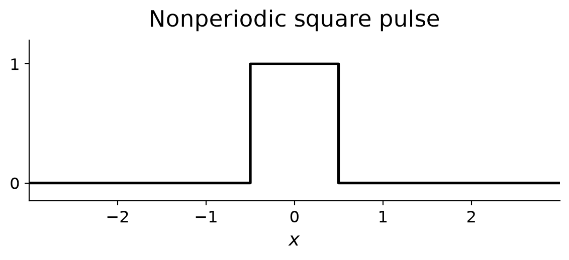
How can we represent a signal that does not repeat?
- Fourier transform: Extends the idea to nonperiodic signals, allowing a continuous range of frequencies.
Fourier Transform Pairs
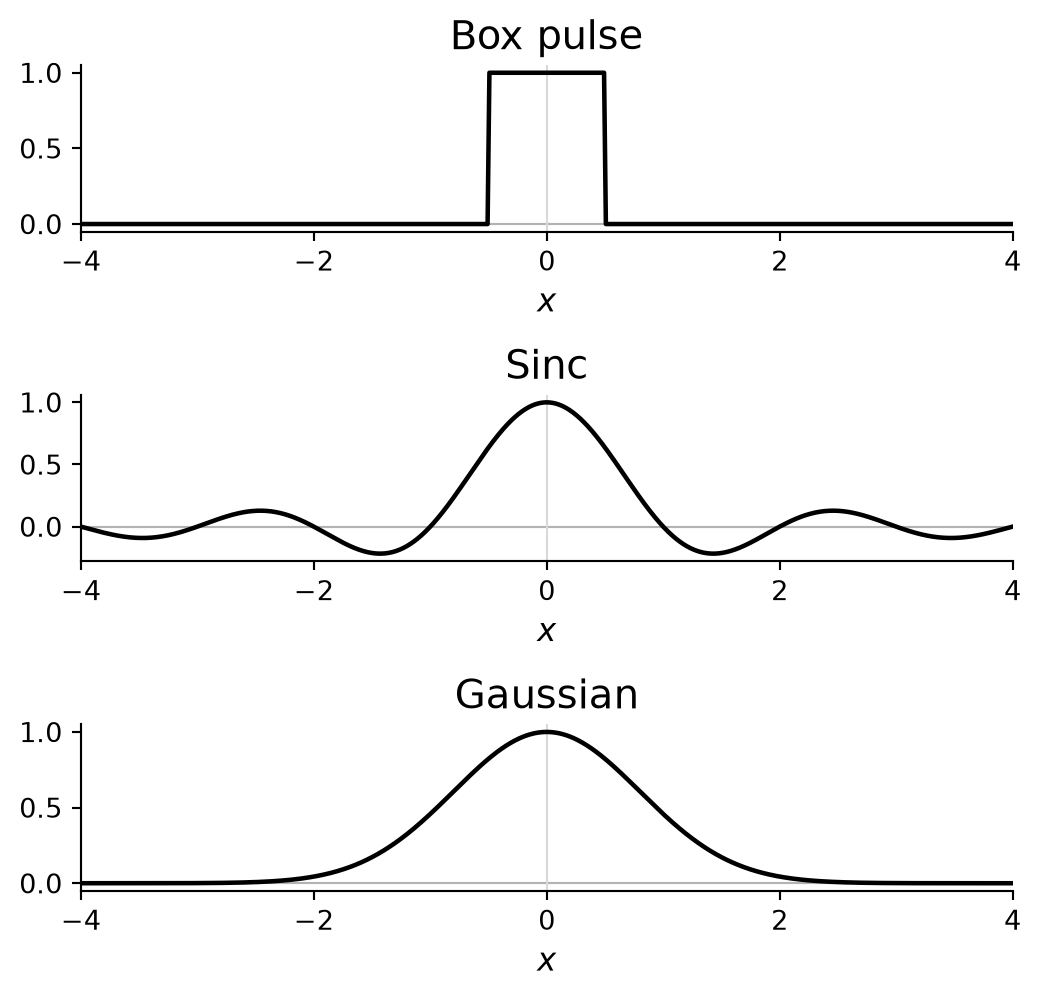
Spatial domain: \(f(x)\)
Frequency domain: \(\operatorname{Re}\{F(\nu)\}\)
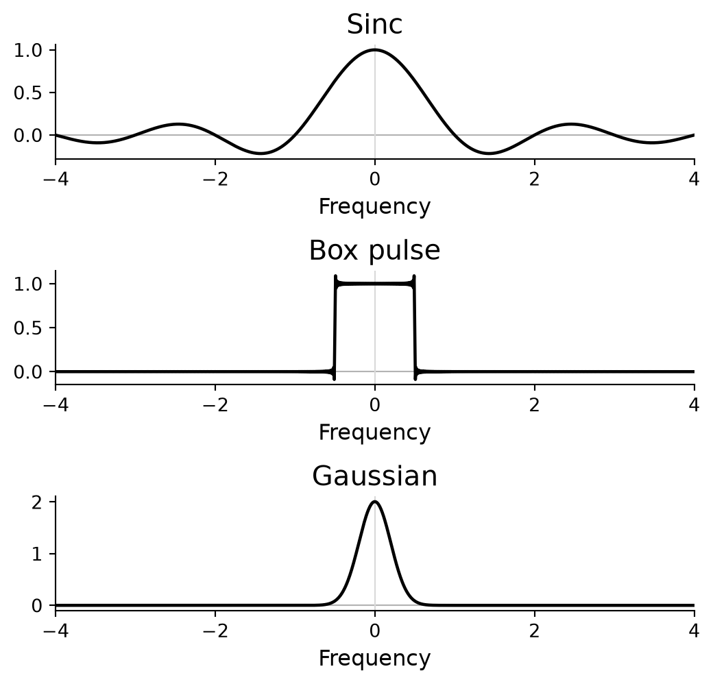
- Box ↔︎ sinc: an example of Fourier-transform duality.
- A Gaussian transforms into another Gaussian; a broader Gaussian produces a narrower spectrum.
Complex Numbers: Cartesian Form
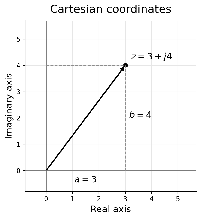
A complex number has two parts:
\[ z = a + jb, \qquad j^2=-1 \]
- \(a\): real part.
- \(b\): imaginary part.
For example:
\[ z=3+j4 \]
The point has coordinates \((a,b)=(3,4)\) in the complex plane.
Complex Numbers: Polar Form
Describe the same point using its distance and angle:
\[ z = r(\cos\theta + j\sin\theta) \]
How do we compute \(r\) and \(\theta\)?
\[ r = |z| = \sqrt{a^2+b^2} \]
\[ \theta = \operatorname{atan2}(b,a) \]
atan2 accounts for the correct quadrant.
For \(z=3+j4\):
\[ r=5, \qquad \theta\approx53.13^\circ \]
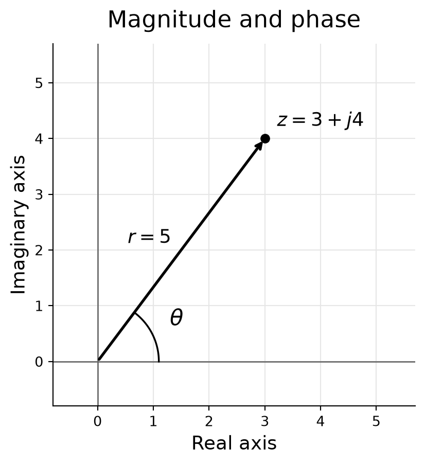
Same complex number, different coordinates: \((a,b)\) or \((r,\theta)\).
Complex Numbers: Exponential Form
Euler’s formula:
\[ e^{j\theta} = \cos\theta + j\sin\theta \]
Therefore:
\[ z = r(\cos\theta+j\sin\theta) = re^{j\theta} \]
- \(r\): magnitude.
- \(\theta\): phase.
For our example, \(\theta\approx0.9273\) radians:
\[ 3+j4 \approx 5e^{j\,0.9273} \]
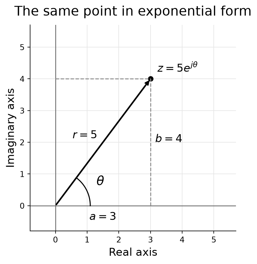
Euler’s formula lets us express the sine and cosine components of the Fourier transform using complex exponentials.
The 2D DFT and Its Inverse
For an image \(I[m,n]\) with \(M\) rows and \(N\) columns:
Forward: image to frequency coefficients
\[ F[v,u] = \sum_{m=0}^{M-1}\sum_{n=0}^{N-1} I[m,n]\, e^{-j2\pi\left(\frac{vm}{M}+\frac{un}{N}\right)} \]
Inverse: frequency coefficients to image
\[ I[m,n] = \frac{1}{MN} \sum_{v=0}^{M-1}\sum_{u=0}^{N-1} F[v,u]\, e^{j2\pi\left(\frac{vm}{M}+\frac{un}{N}\right)} \]
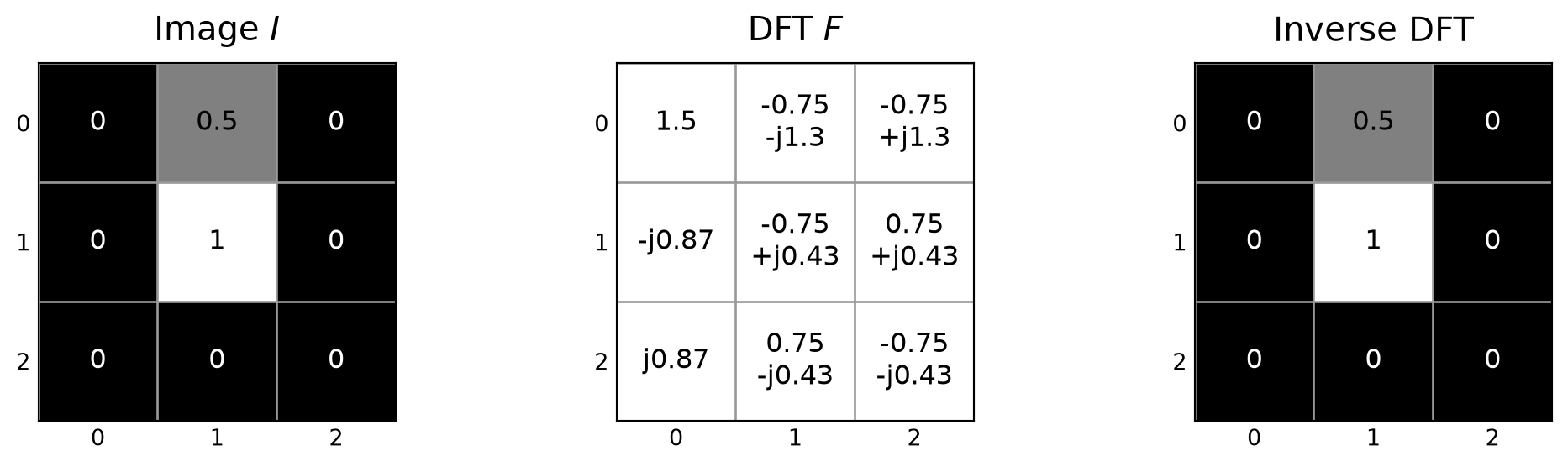
- Nine pixel values become nine complex coefficients.
- The inverse recovers exactly the same original pixel values.
Computing the Image DFT with Matrices
For our \(3\times3\) image, set \(N=3\) in the DFT matrix:
\[ \mathbf{W}_3 = \begin{bmatrix} 1 & 1 & 1\\ 1 & \omega & \omega^2\\ 1 & \omega^2 & \omega \end{bmatrix}, \qquad \omega=e^{-j2\pi/3} \]
Here \(\omega^3=1\), so \(\omega^4=\omega\).
\[ \underbrace{\mathbf{B}=\mathbf{I}\mathbf{W}_3^T} _{\text{Transform each row}} \qquad \underbrace{\mathbf{F}=\mathbf{W}_3\mathbf{B}} _{\text{Transform each column}} \]
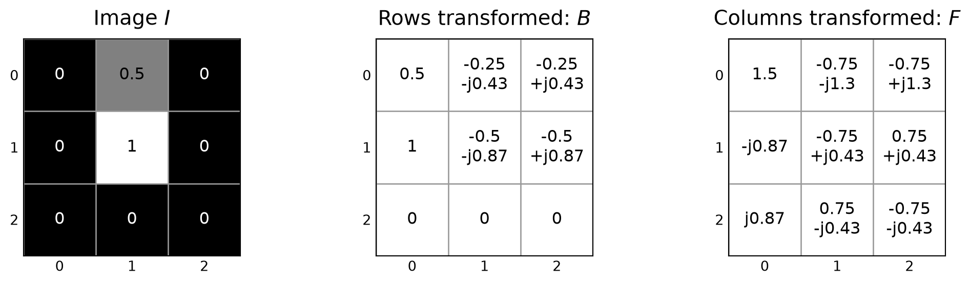
These are the same Fourier coefficients as before, computed using row and column transforms.
Magnitude and Phase of the Same Transform
At each frequency, the same coefficient has two representations:
Cartesian form:
\[ F=a+jb \]
- Real part: \(a=\operatorname{Re}\{F\}\).
- Imaginary part: \(b=\operatorname{Im}\{F\}\).
Polar form:
\[ F=Ae^{j\theta} \]
- Magnitude: \(A=|F|=\sqrt{a^2+b^2}\).
- Phase: \(\theta=\operatorname{atan2}(b,a)\).

Magnitude and phase together retain the information needed for reconstruction.
Computing an Image DFT with OpenCV
import cv2
import numpy as np
import matplotlib.pyplot as plt

I = cv2.imread("assets/05_fourier_transform/co_logo.png",
               cv2.IMREAD_GRAYSCALE)

I = cv2.resize(I, (64, 64), interpolation=cv2.INTER_AREA)
I = I.astype(np.float32) / 255
H, W = I.shape

F_raw = cv2.dft(I, flags=cv2.DFT_COMPLEX_OUTPUT)
F = np.roll(F_raw, (H//2, W//2), axis=(0, 1))

a, b = F[:, :, 0], F[:, :, 1]
A, theta = cv2.cartToPolar(a, b)
theta = np.where(theta > np.pi, theta - 2*np.pi, theta)
theta[A == 0] = np.nan

# Compress contrast for display only.
real_view = np.sign(a) * np.log1p(np.abs(a))
imag_view = np.sign(b) * np.log1p(np.abs(b))
L = max(np.abs(real_view).max(), np.abs(imag_view).max())

views = [I, real_view, imag_view, np.log1p(A), theta]
titles = ["Image", "Real (signed log)", "Imaginary (signed log)",
          "Magnitude (log)", "Phase"]
limits = [(0, 1), (-L, L), (-L, L), (0, None), (-np.pi, np.pi)]

fig, ax = plt.subplots(2, 3, figsize=(8.2, 6))
for axis, view, title, (lo, hi) in zip(ax.flat, views, titles, limits):
    axis.imshow(view, cmap="gray", vmin=lo, vmax=hi,
                interpolation="nearest")
    axis.set_title(title, fontsize=14)
    axis.axis("off")
ax.flat[-1].axis("off")

fig.tight_layout()
plt.show()
plt.close(fig)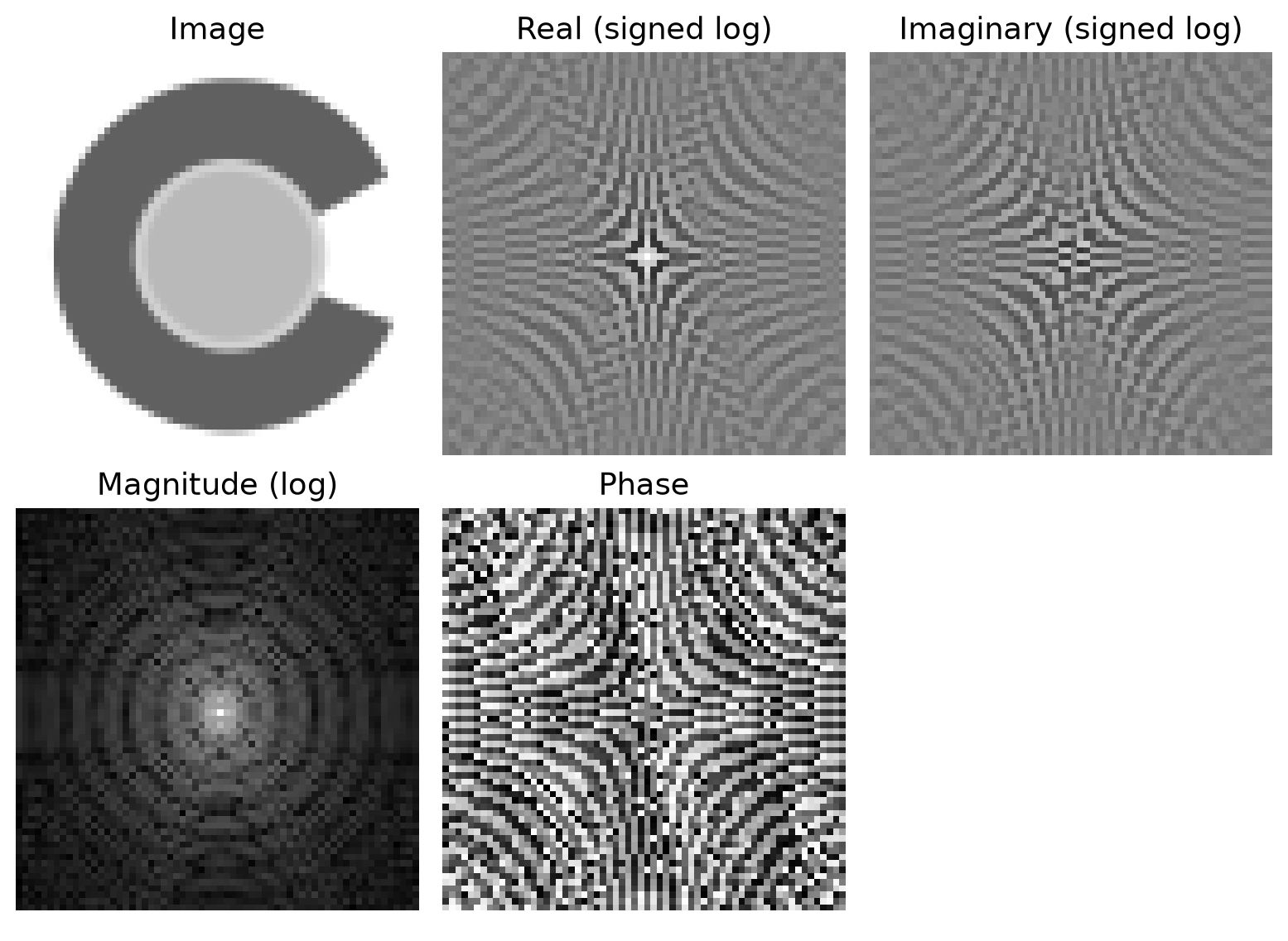
Why Center the Fourier Spectrum?
OpenCV stores the zero-frequency coefficient at the upper-left corner.
For visualization, the convention is to move it to the center.
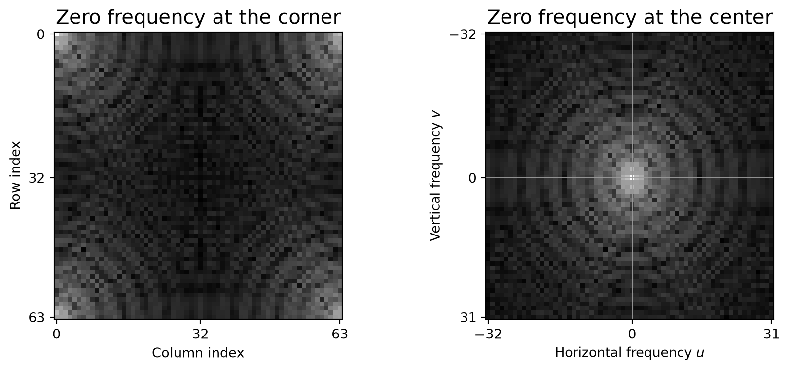
- The center represents zero frequency, with positive and negative frequencies on opposite sides.
- Frequencies farther from the center represent more rapid intensity changes.
- Centering rearranges the coefficients; it does not change their values or the original image’s pixel coordinates.
Reading a Fourier Spectrum
How do these images appear in the spectrum?
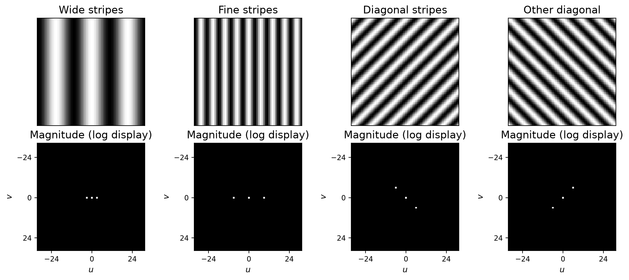
- Finer stripes: the two side peaks move farther from the center.
- Orientation: the line joining the peaks is perpendicular to the stripes.
- Center peak: these images have a nonzero mean intensity.
Two Extremes: A Point and a Constant Image
What frequencies are needed to represent each image?
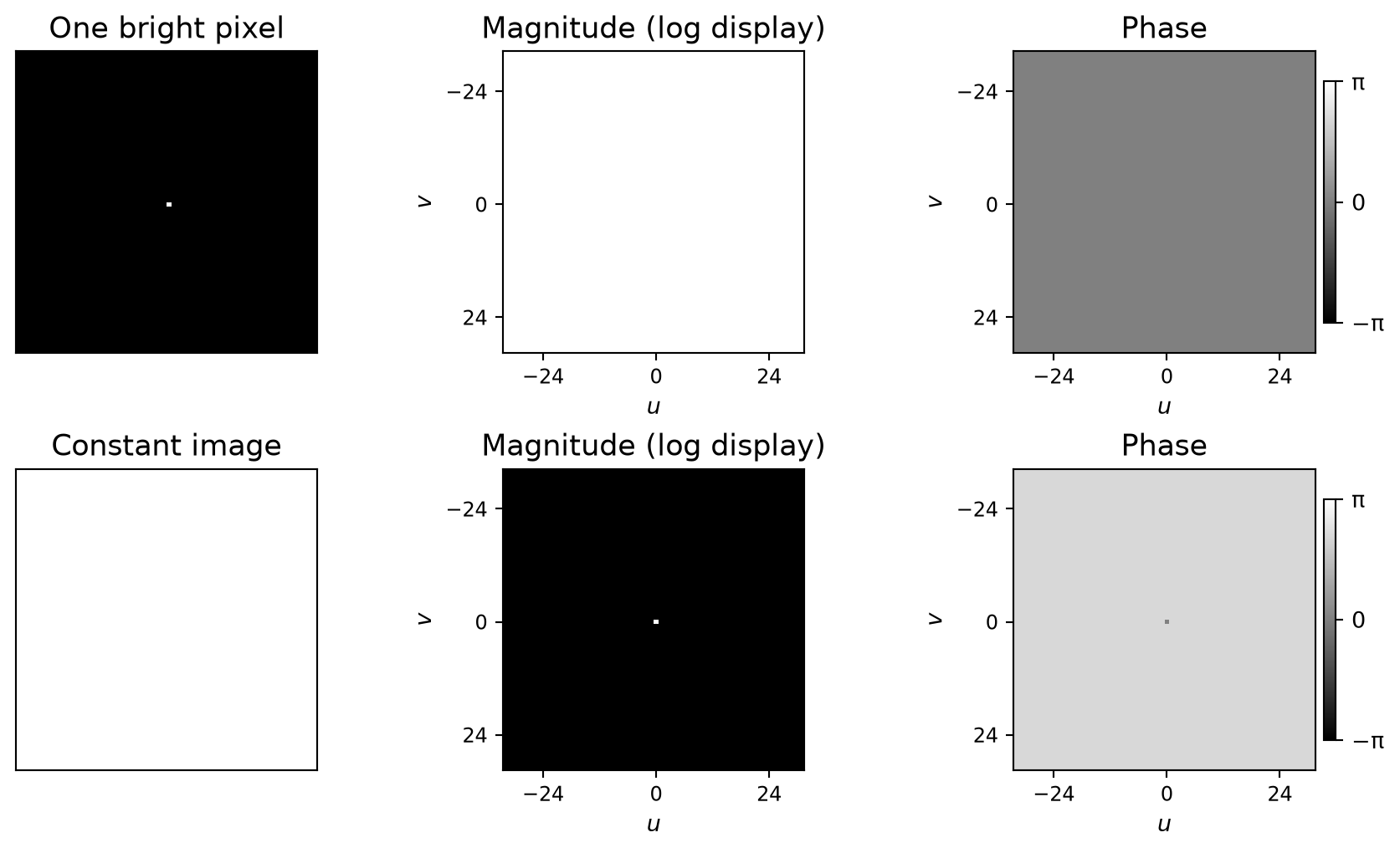
- One bright pixel: all frequencies contribute equally; every DFT magnitude is \(1\).
- Constant image: only the zero-frequency component remains; its value is the number of pixels in the image.
From a Point to a Line
A horizontal line is constant horizontally, but changes sharply vertically.
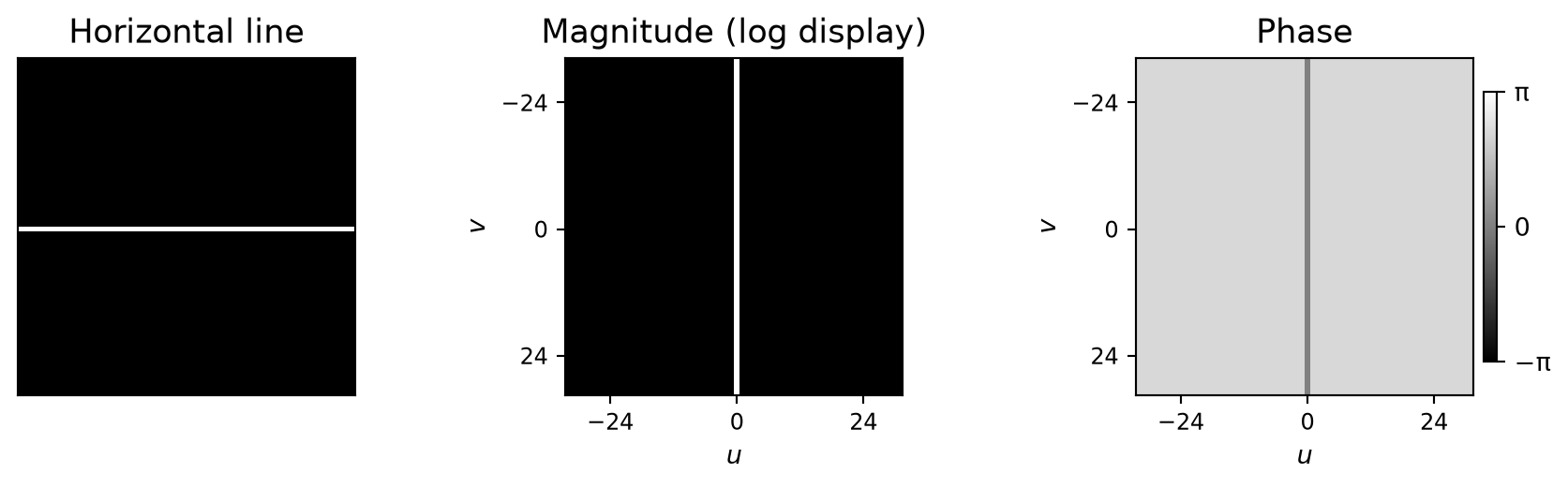
Along the line
There is no horizontal variation.
Only the horizontal frequency \(u=0\) is needed.
Across the line
A one-pixel change requires all vertical frequencies.
The spectrum extends along the \(v\) axis.
A horizontal line produces a vertical line in the Fourier magnitude.
Repeated Points Produce Repeated Peaks
A regular grid of bright pixels is called an impulse train or impulse comb.
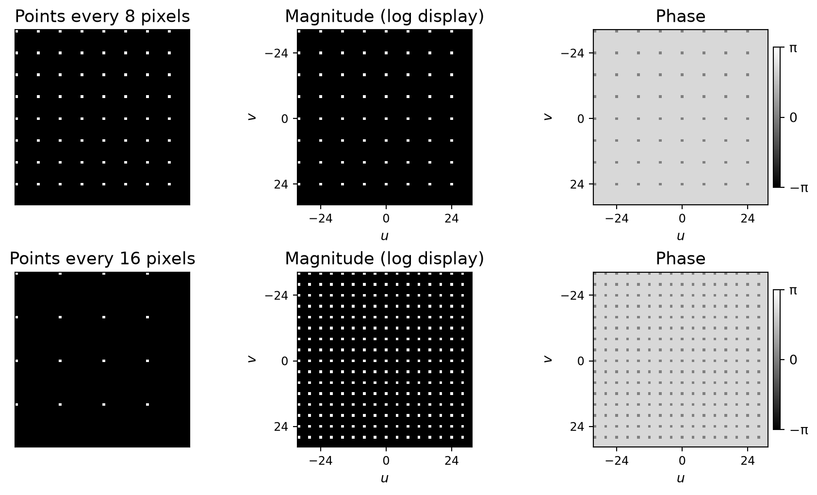
- A regular grid in the image produces a regular grid in the spectrum.
- Farther-apart points → closer-together frequency peaks.
Translation Changes Phase, Not Magnitude
Move the square without changing its shape or brightness.
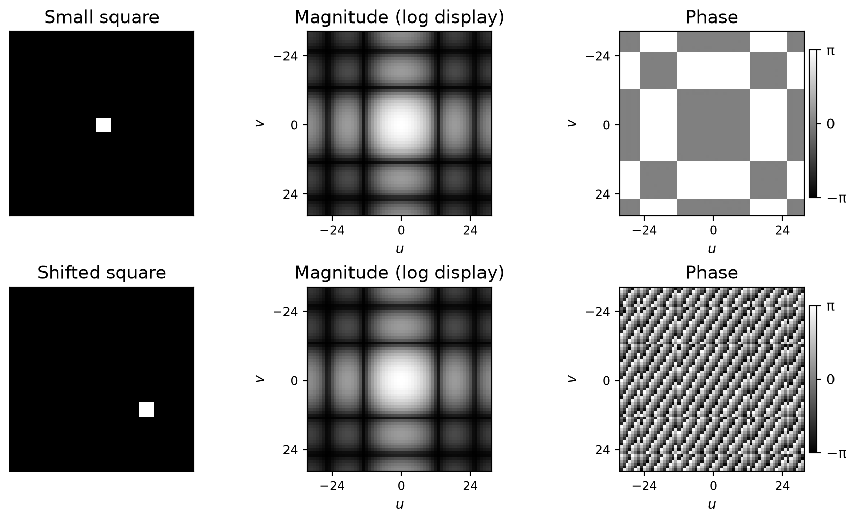
- The magnitude stays the same: the same frequencies are present.
- The phase changes: the waves must align at a different location.
- Magnitude alone cannot tell us where the square is located.
Spatial Size and Frequency Spread
Compare the same shape at two different sizes.
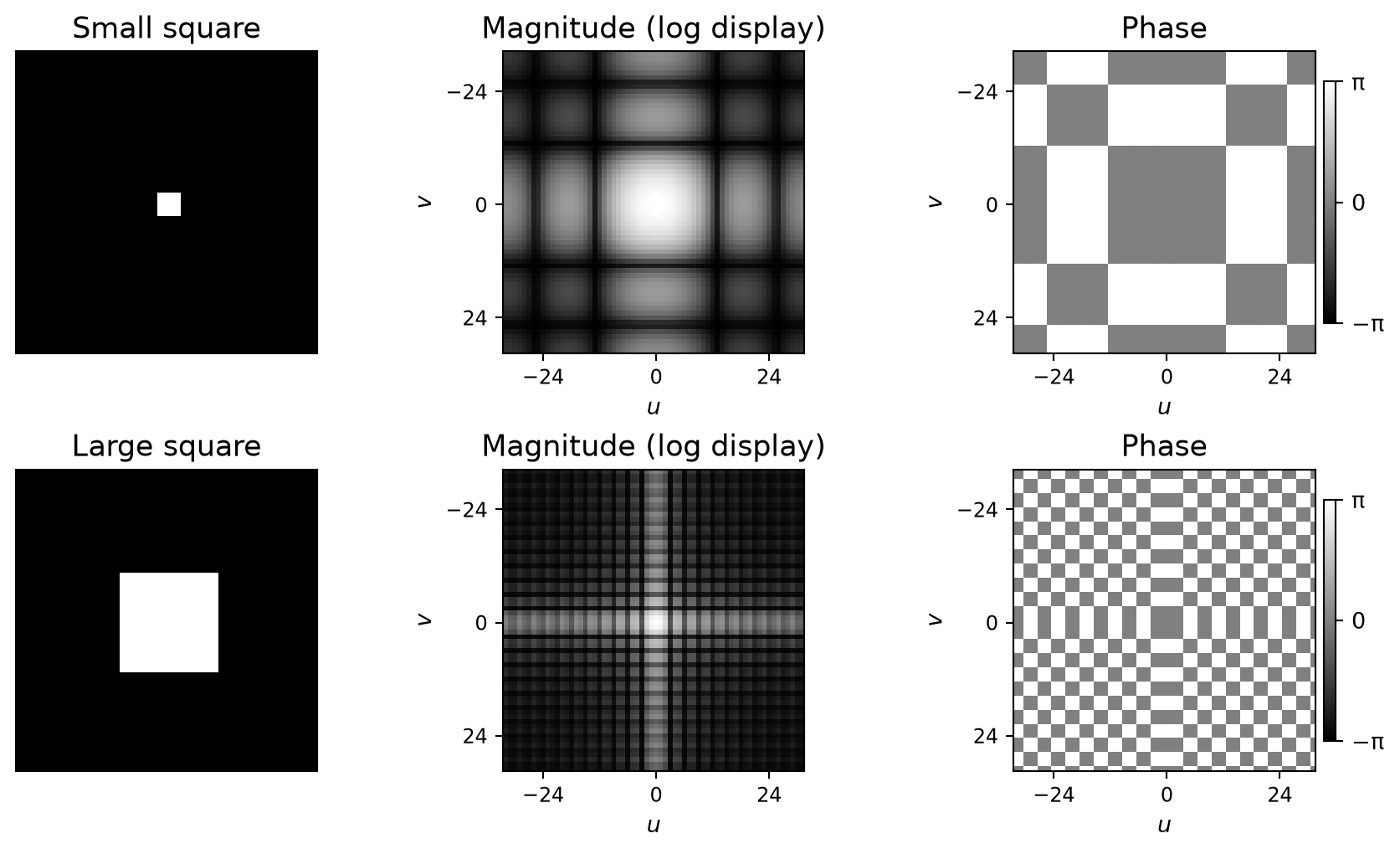
- Smaller square → broader central lobe in the spectrum.
- Larger square → narrower central lobe.
- Spatial extent and frequency spread have an inverse relationship.
Rotating an Image Rotates Its Spectrum
The spectrum follows the orientation of the image.
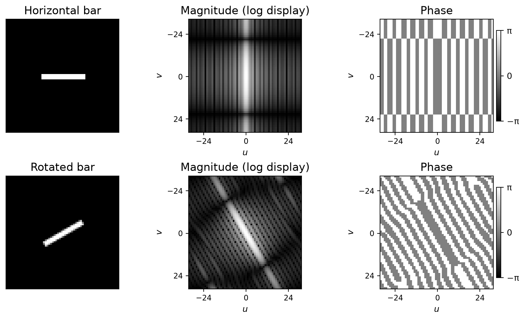
- Rotating the bar rotates this frequency pattern by the same angle.
Quiz: Match Each Image to Its Fourier Spectrum
Match images A–H to the centered DFT amplitudes 1–8.
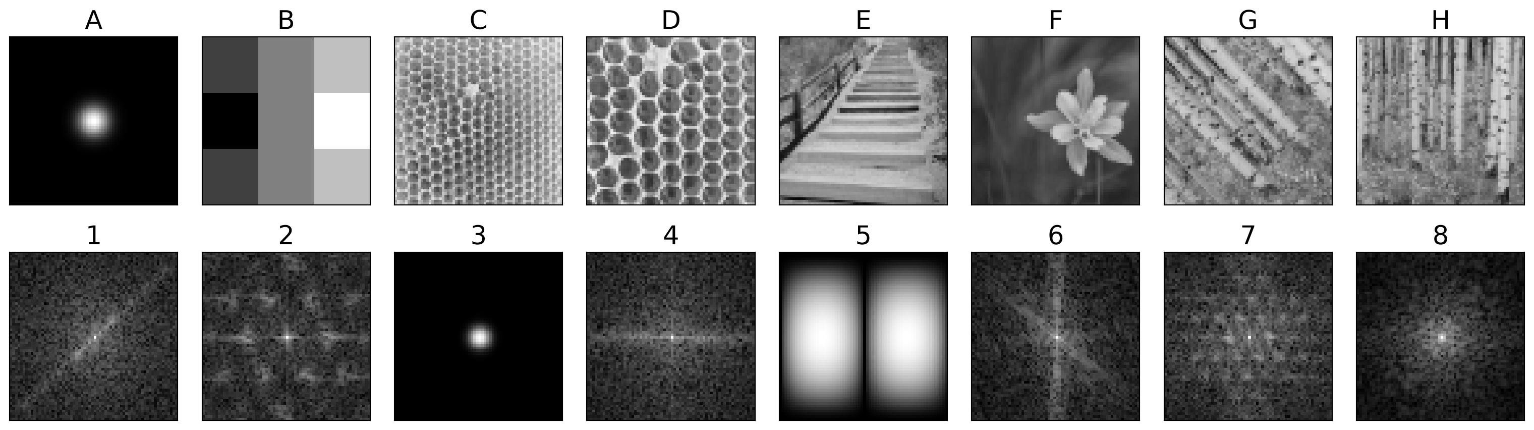
Explain your matches using frequency spread, orientation, and repeated patterns.
Reconstructing an Image from Fourier Coefficients
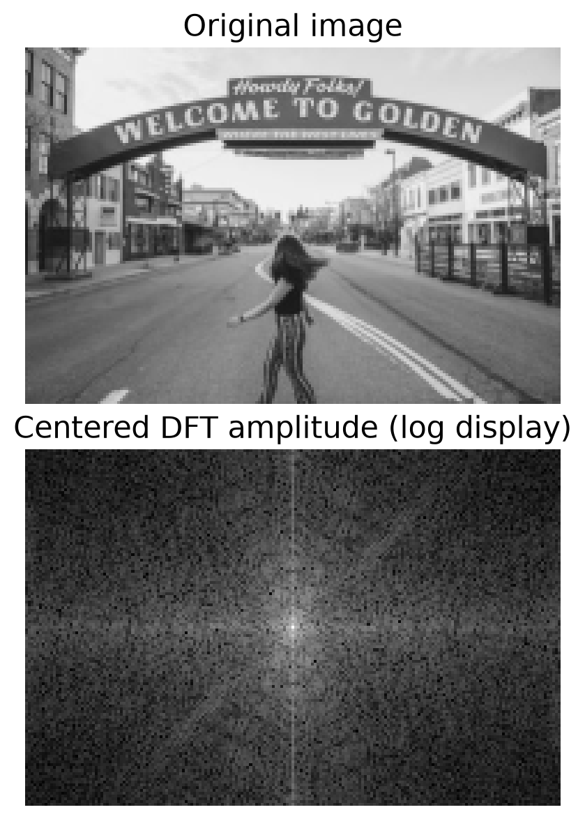
The inverse DFT reconstructs the image:
\[ I = \mathcal{F}^{-1}(F). \]
What if we retain only some coefficients?
- Keep the selected complex values.
- Set every other coefficient to zero.
- Apply the inverse DFT.
\[ \widehat{I}_K = \mathcal{F}^{-1}(M_K \odot F) \]
Here, \(M_K\) is a binary mask selecting \(K\) coefficients.
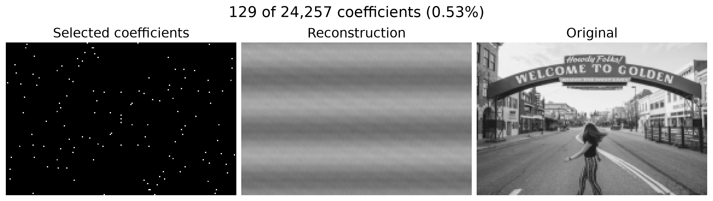
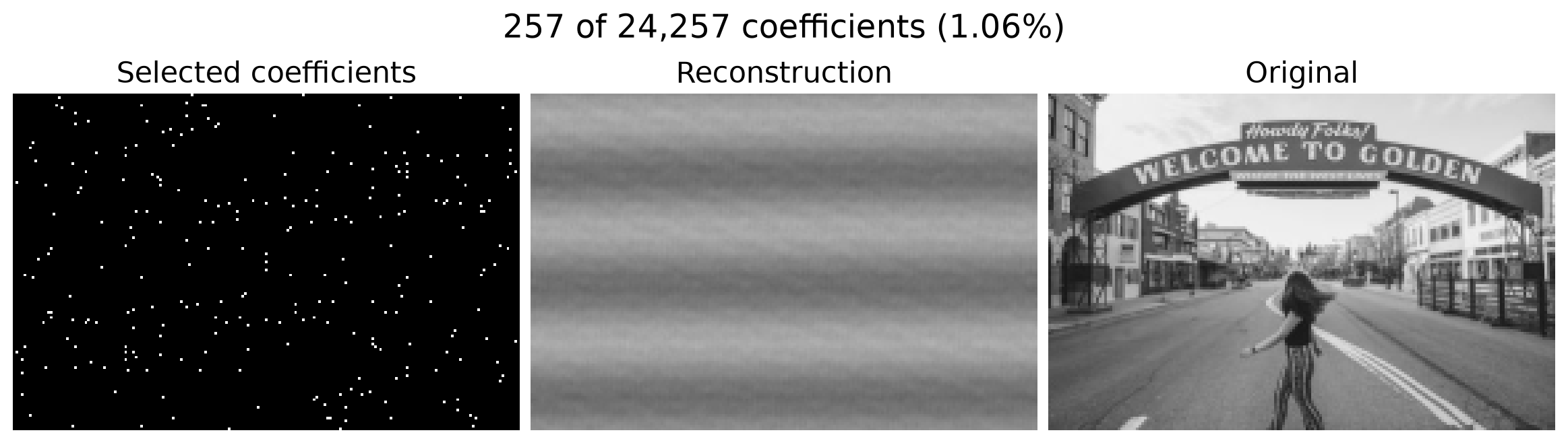
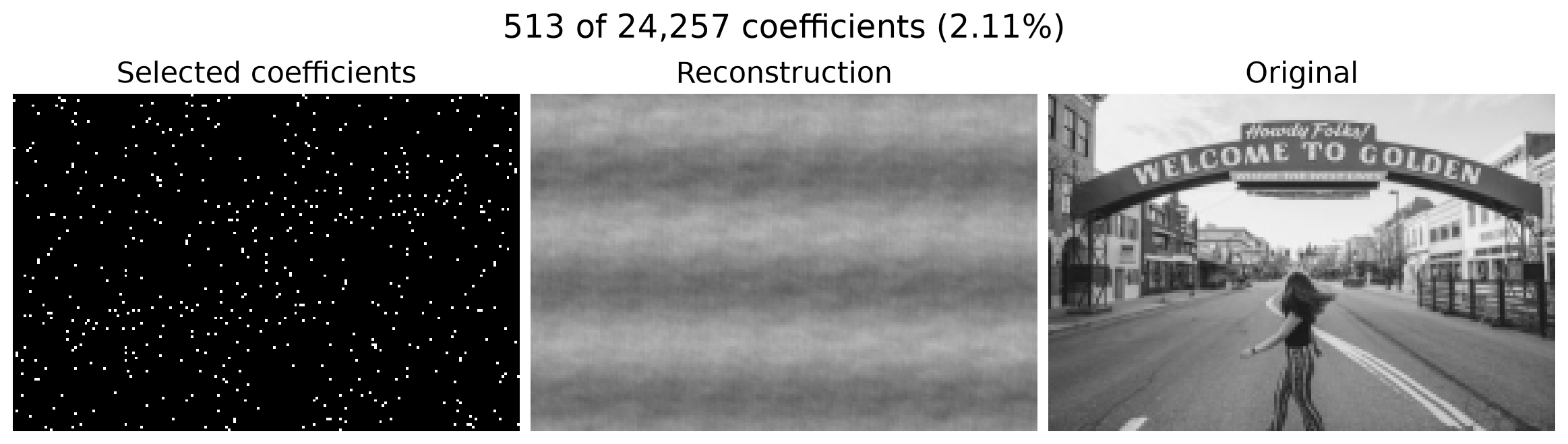
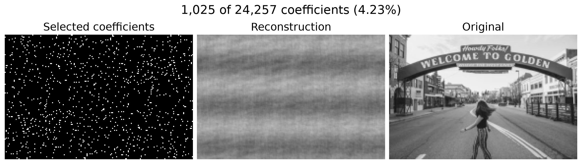
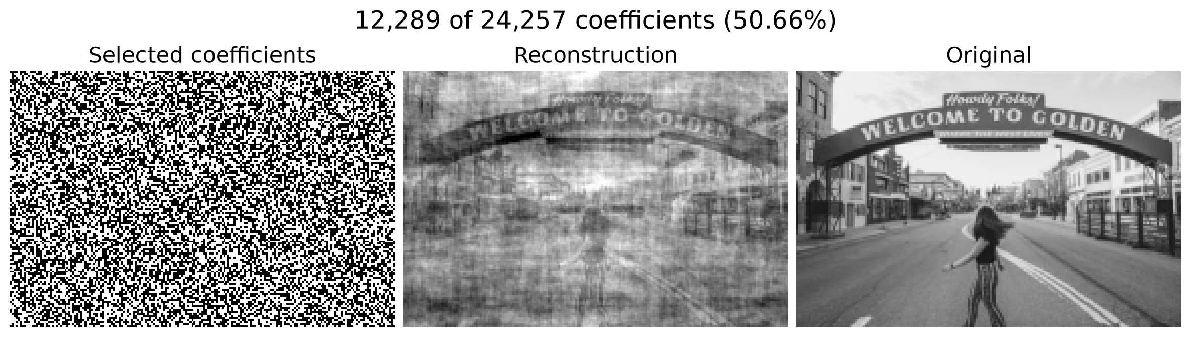
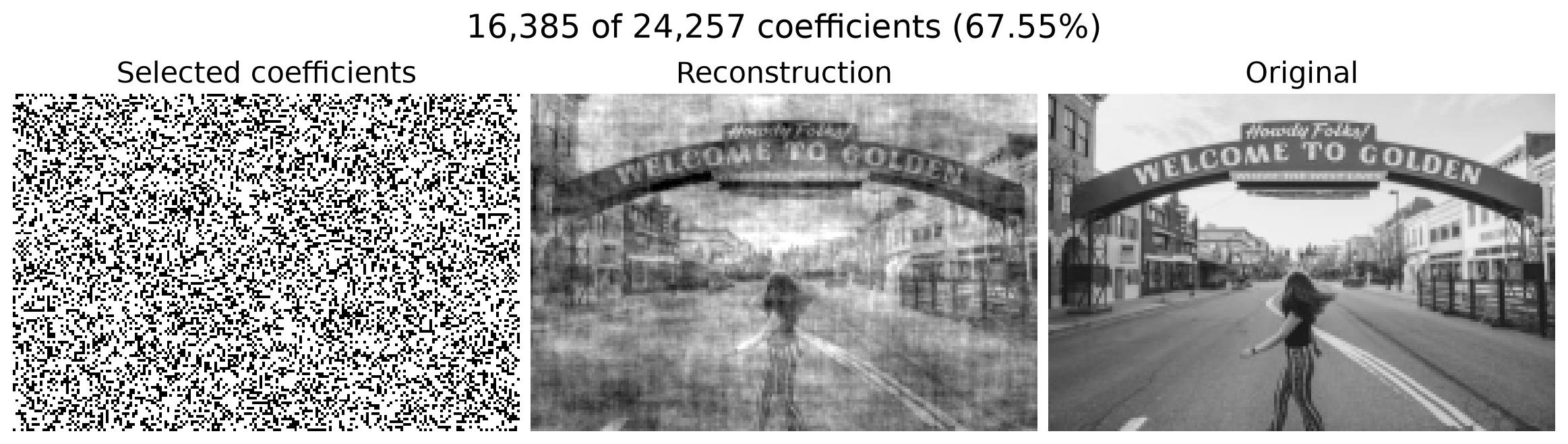
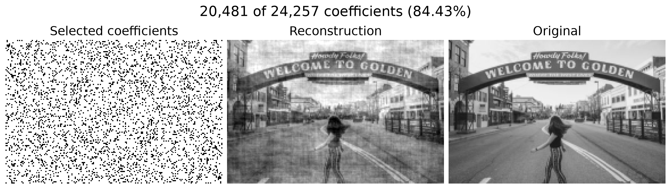
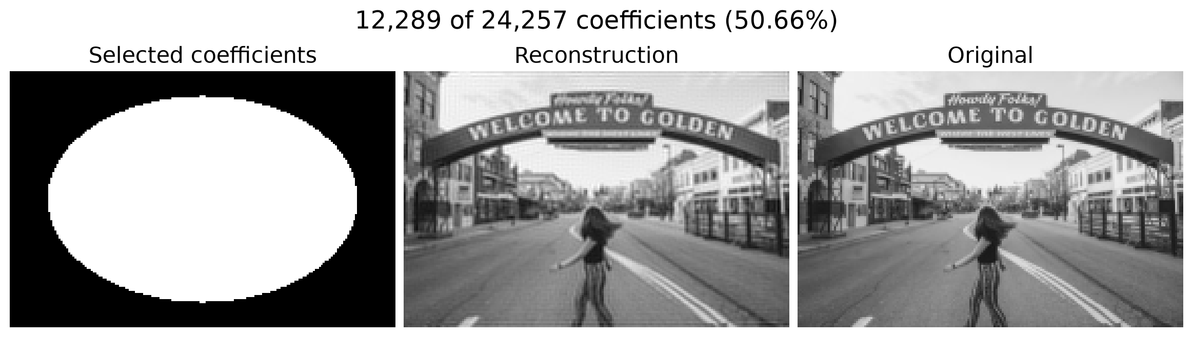
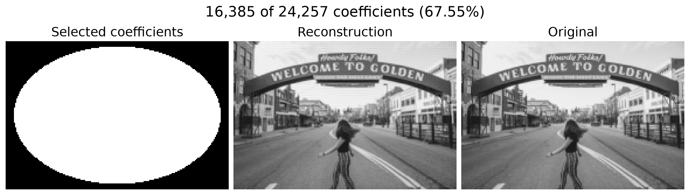
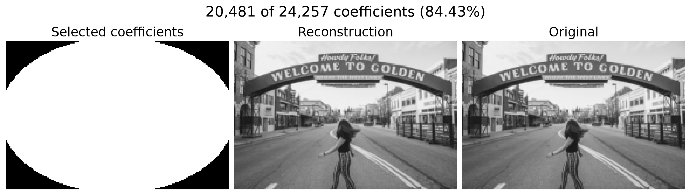
Which selection works better: random frequencies or frequencies near the center?
Random Selection: 1 Coefficient
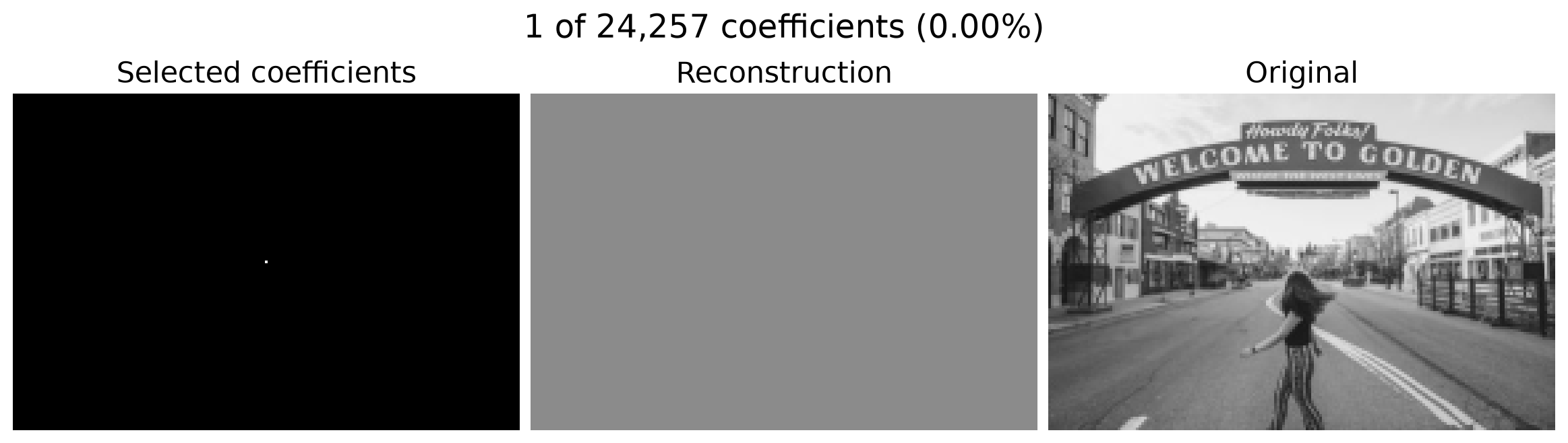
Only DC remains: every pixel equals the original image’s mean intensity.
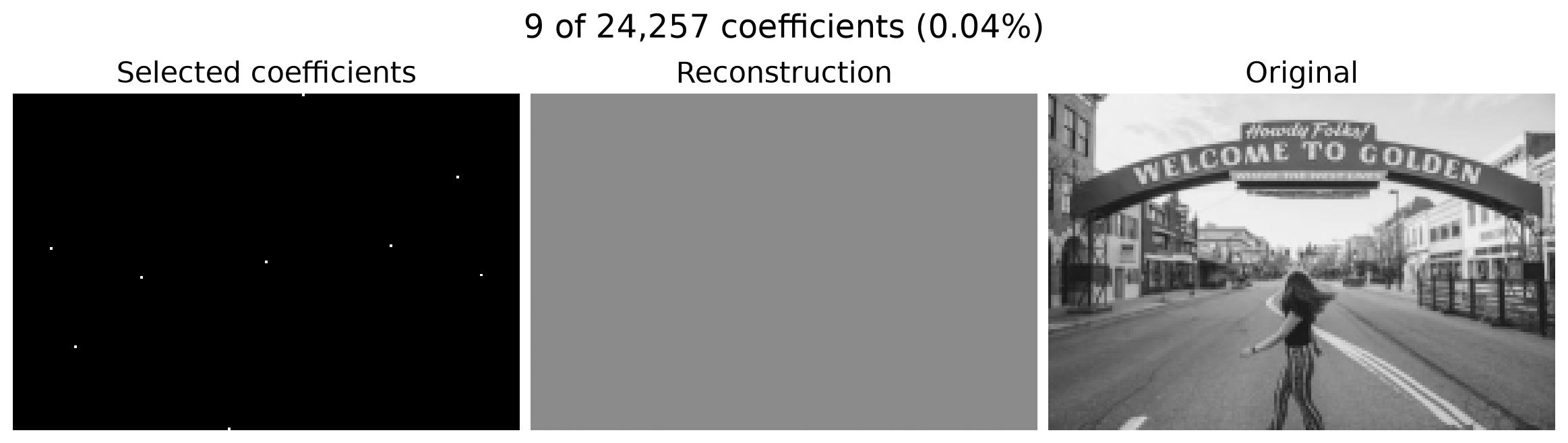
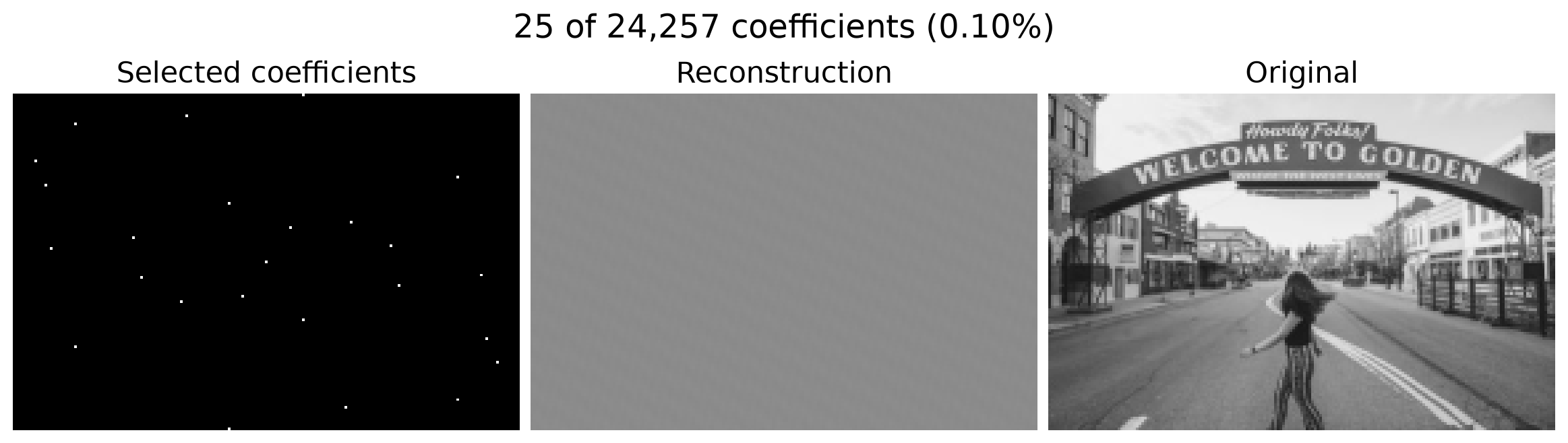
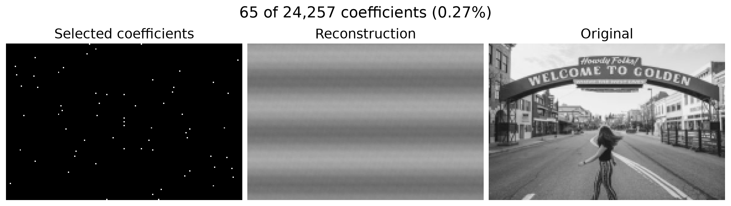
White pixels in the mask mark retained coefficients; black pixels mark discarded coefficients.
Random Selection: 9 Coefficients
Random Selection: 25 Coefficients
Random Selection: 65 Coefficients
Random Selection: 129 Coefficients
Random Selection: 257 Coefficients
Random Selection: 513 Coefficients
Random Selection: 1,025 Coefficients
Random Selection: 2,049 Coefficients
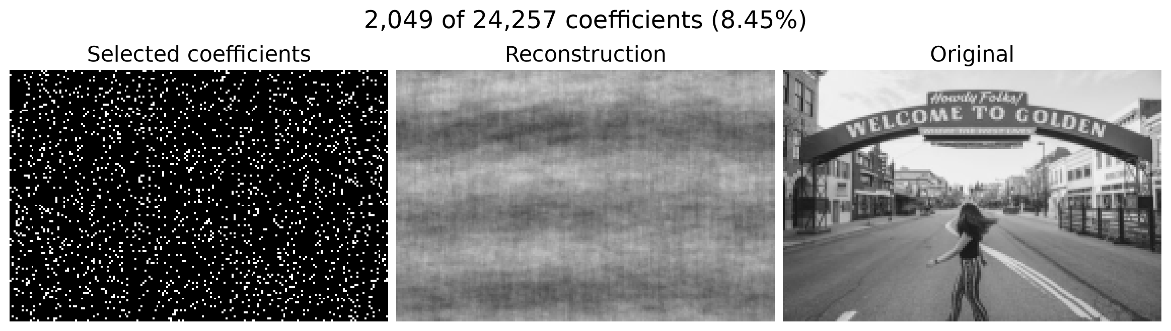
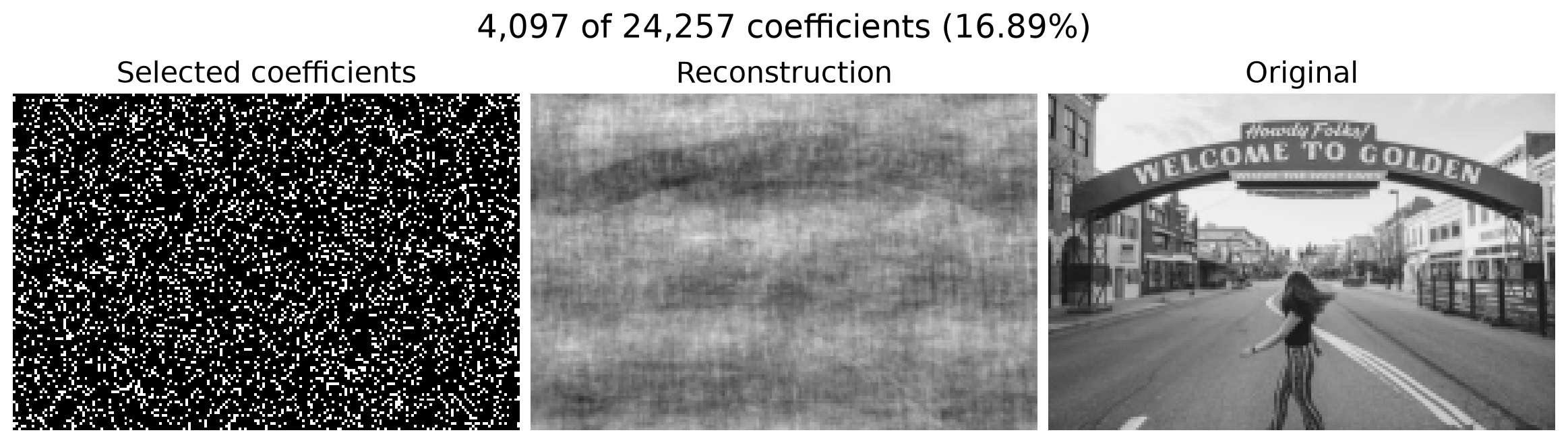
Random Selection: 4,097 Coefficients
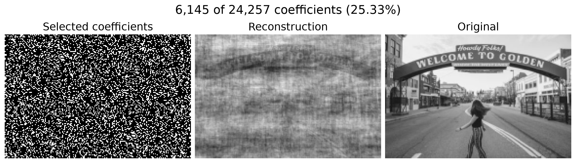
Random Selection: 6,145 Coefficients
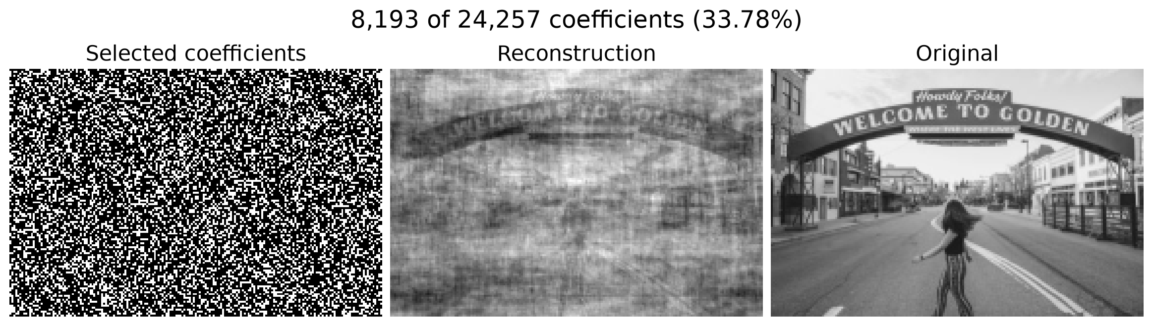
Random Selection: 8,193 Coefficients
Random Selection: 12,289 Coefficients
Random Selection: 16,385 Coefficients
Random Selection: 20,481 Coefficients
Random Selection: All 24,257 Coefficients
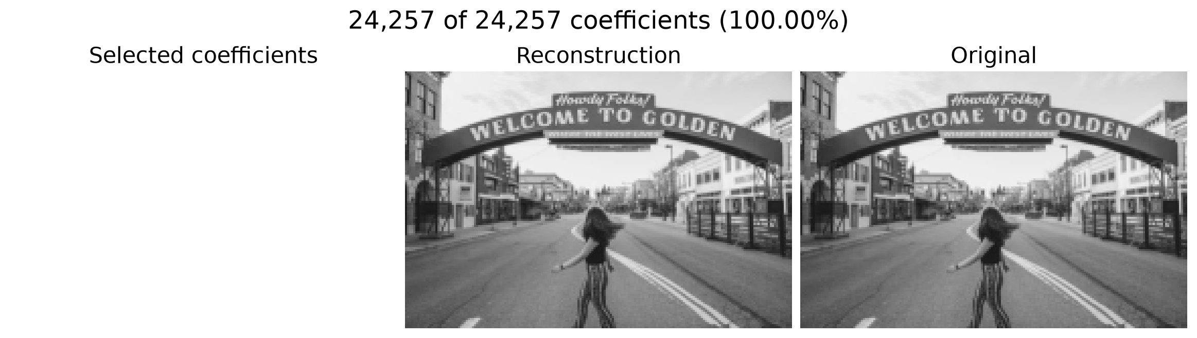
With all coefficients retained, the inverse DFT recovers the original image.
Can we obtain a useful reconstruction with far fewer coefficients?
Selecting from the Center: 1 Coefficient
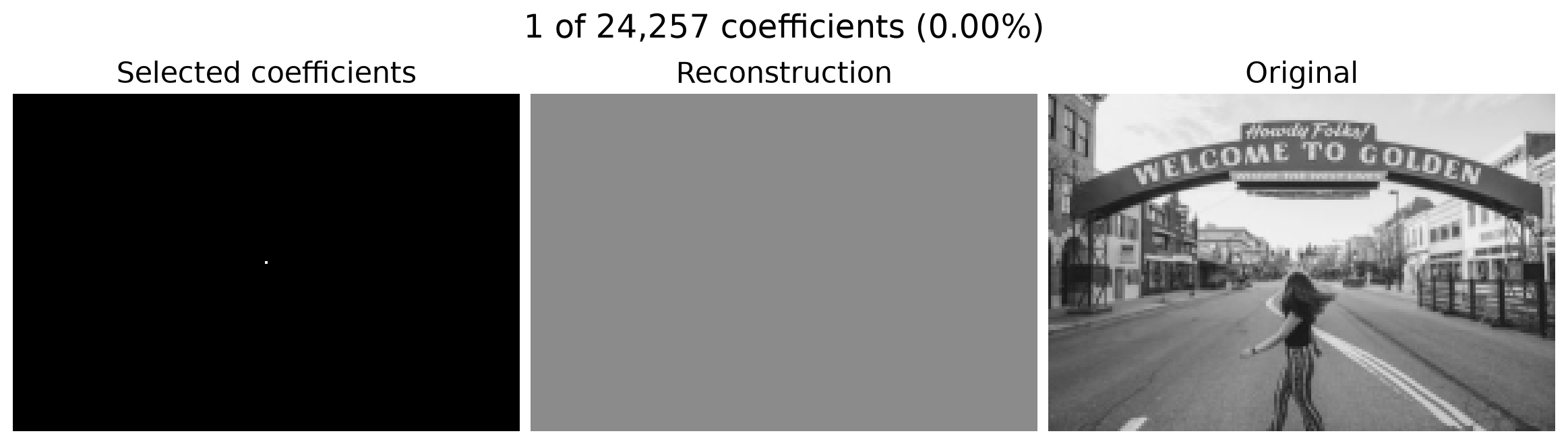
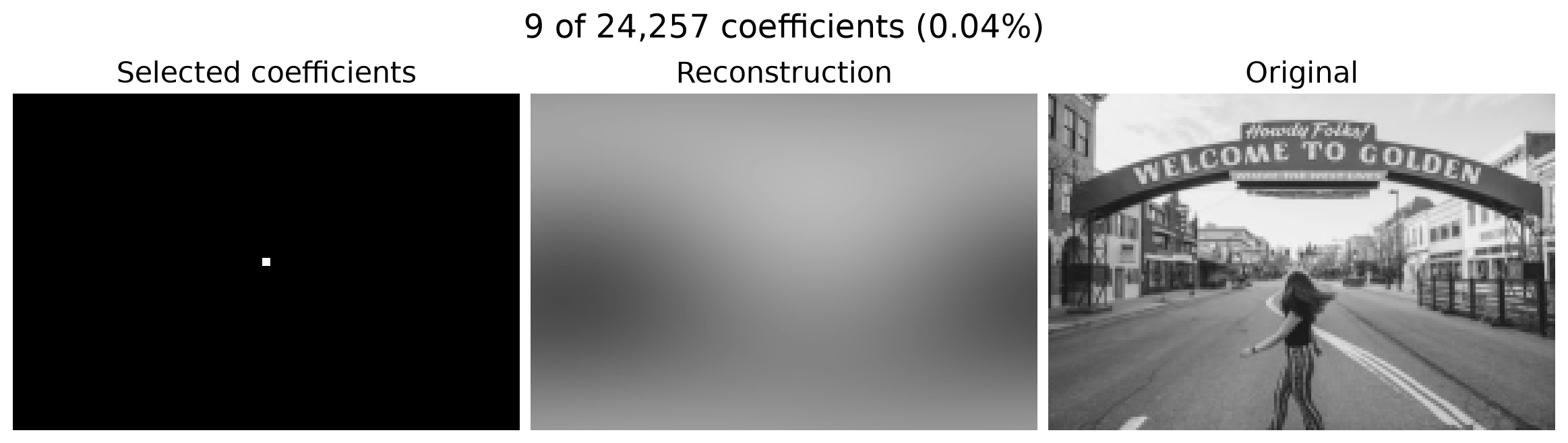
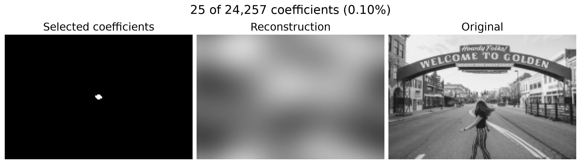
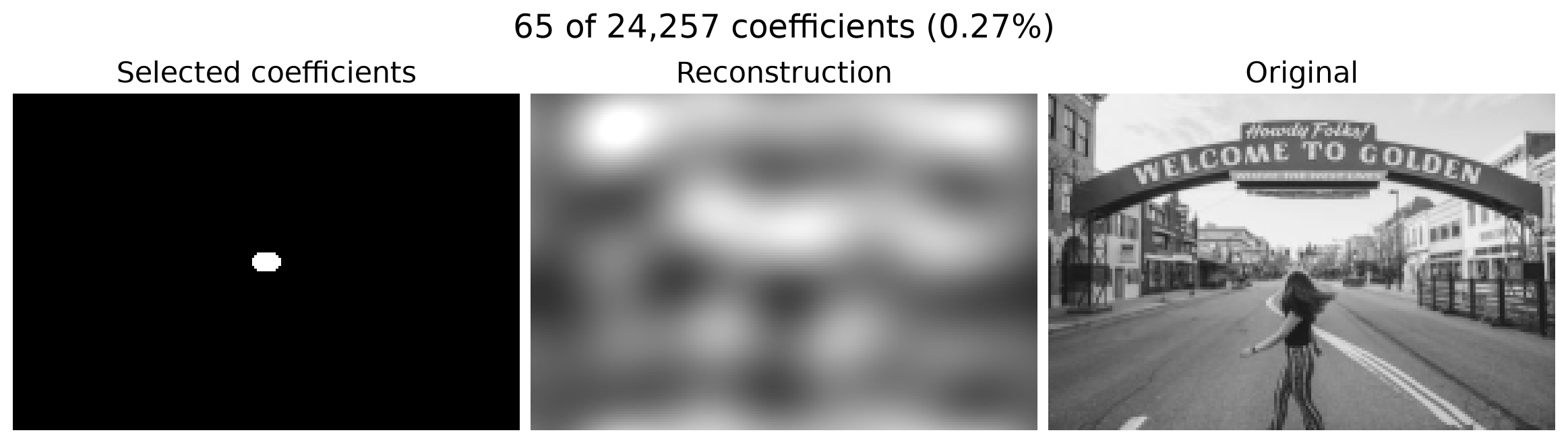
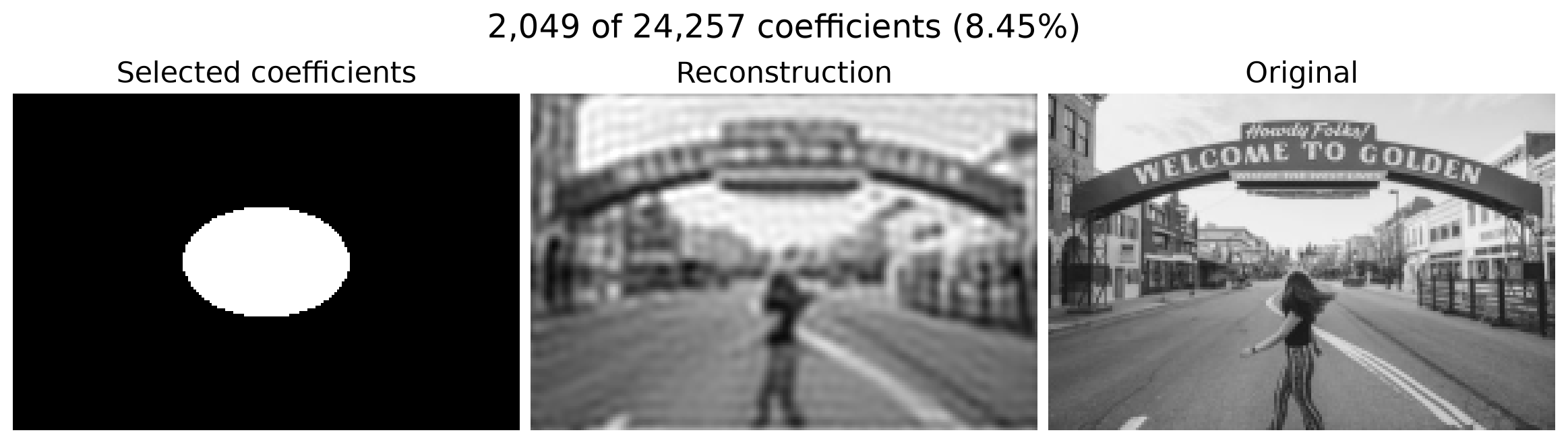
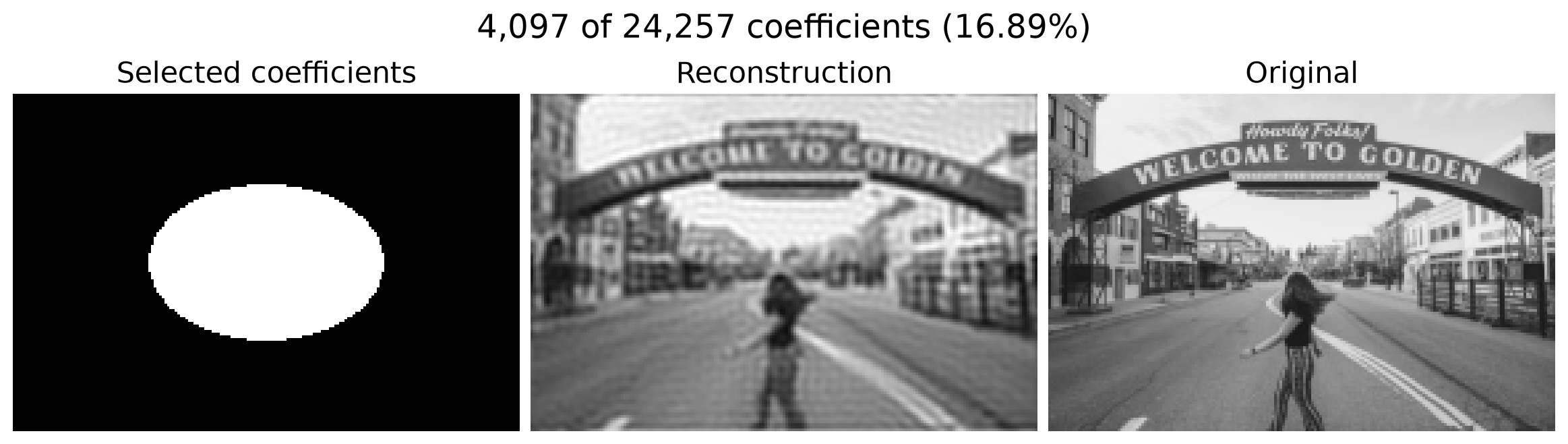
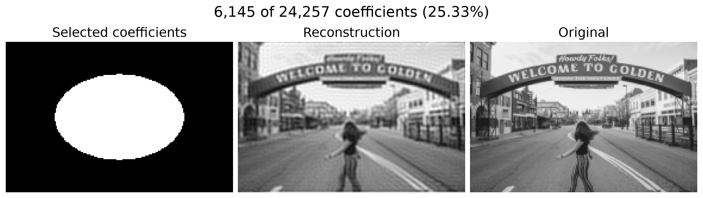
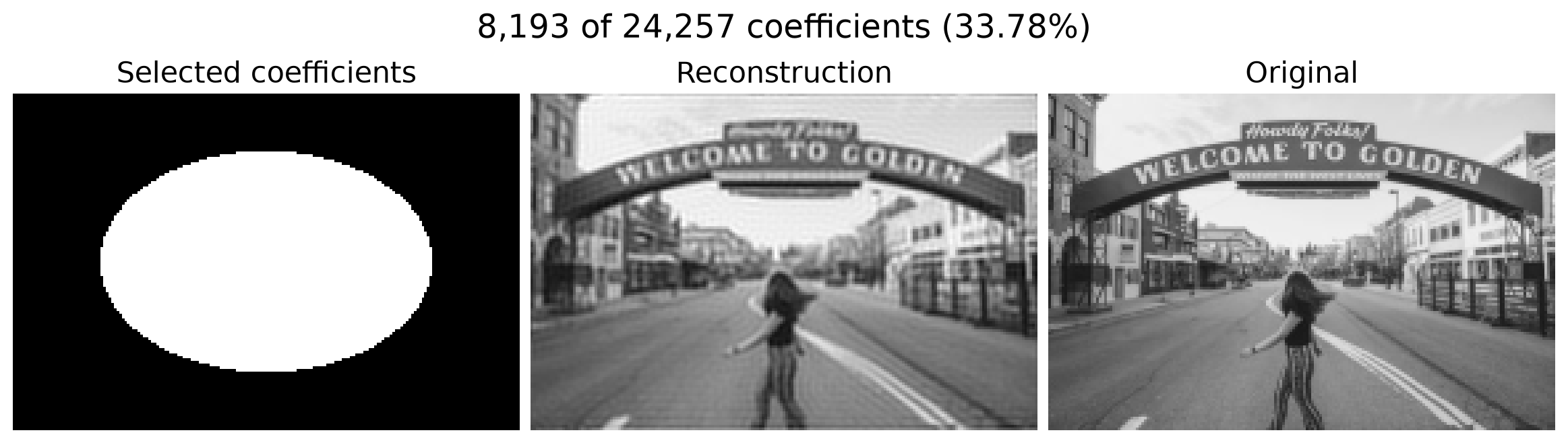
Start with DC, then expand outward to include progressively higher frequencies.
We will use the same coefficient counts as before.
Selecting from the Center: 9 Coefficients
Selecting from the Center: 25 Coefficients
Selecting from the Center: 65 Coefficients
Selecting from the Center: 129 Coefficients
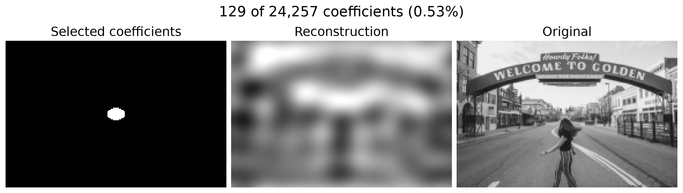
Selecting from the Center: 257 Coefficients
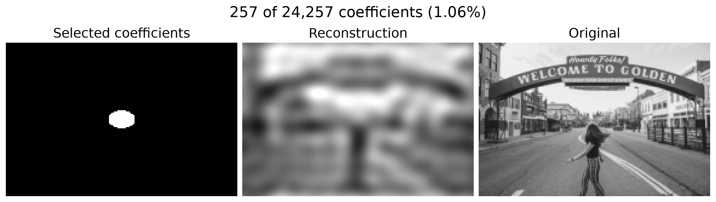
Selecting from the Center: 513 Coefficients
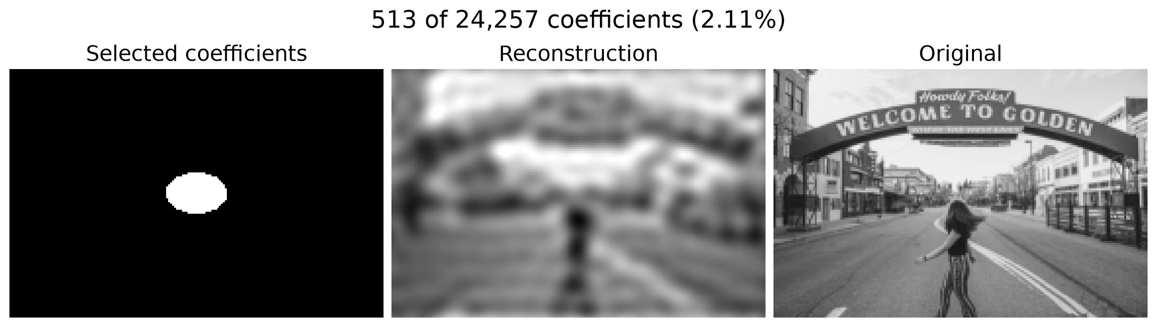
Selecting from the Center: 1,025 Coefficients
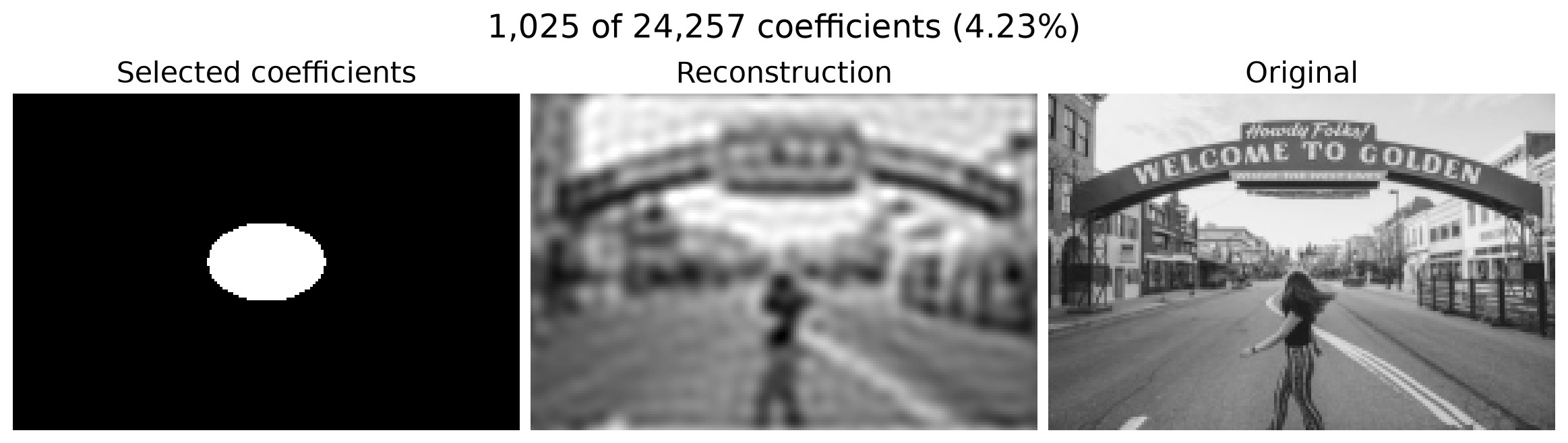
The scene is already recognizable using about 4.2% of the coefficients.
Selecting from the Center: 2,049 Coefficients
Selecting from the Center: 4,097 Coefficients
Selecting from the Center: 6,145 Coefficients
Selecting from the Center: 8,193 Coefficients
Selecting from the Center: 12,289 Coefficients
Selecting from the Center: 16,385 Coefficients
Selecting from the Center: 20,481 Coefficients
Selecting from the Center: All 24,257 Coefficients
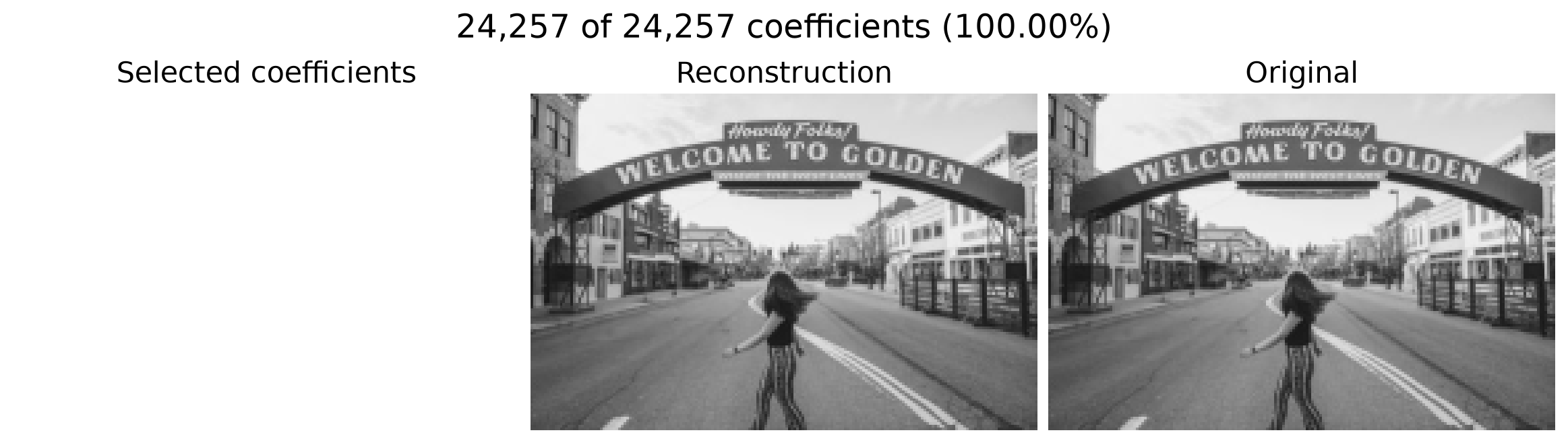
Both methods reach the same exact reconstruction when all coefficients are retained.
Same Number of Coefficients, Different Results
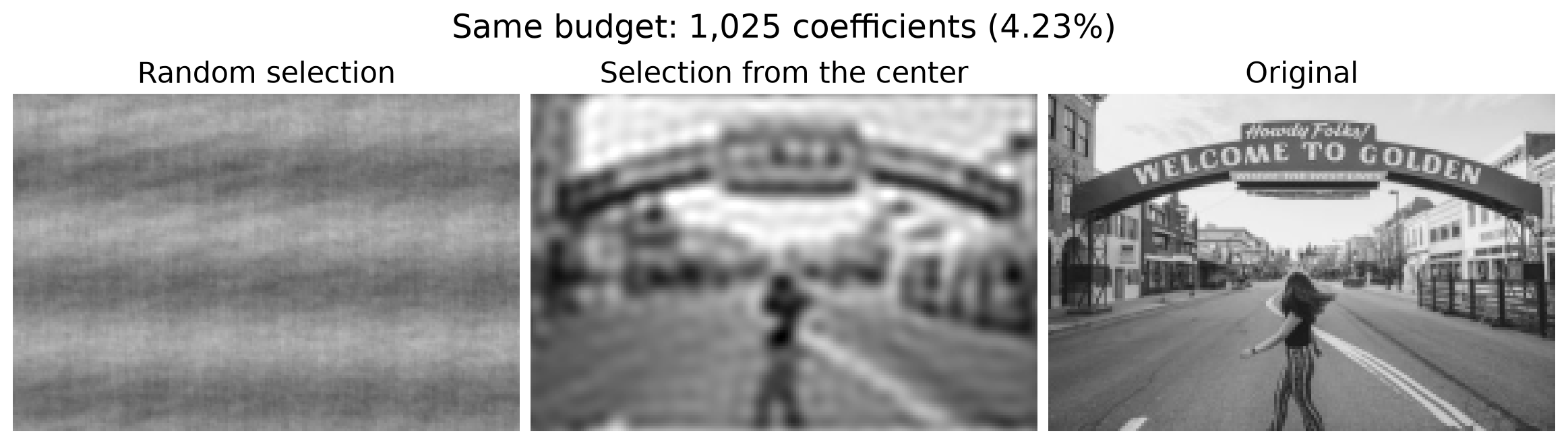
- Low frequencies capture much of this image’s broad structure.
- Adding higher frequencies restores sharper edges and finer details.
- Random selection spends many coefficients on frequencies that contribute little to this image.
Compression idea: retain informative transform coefficients and encode them efficiently.
Where Is the Energy in Natural Images?
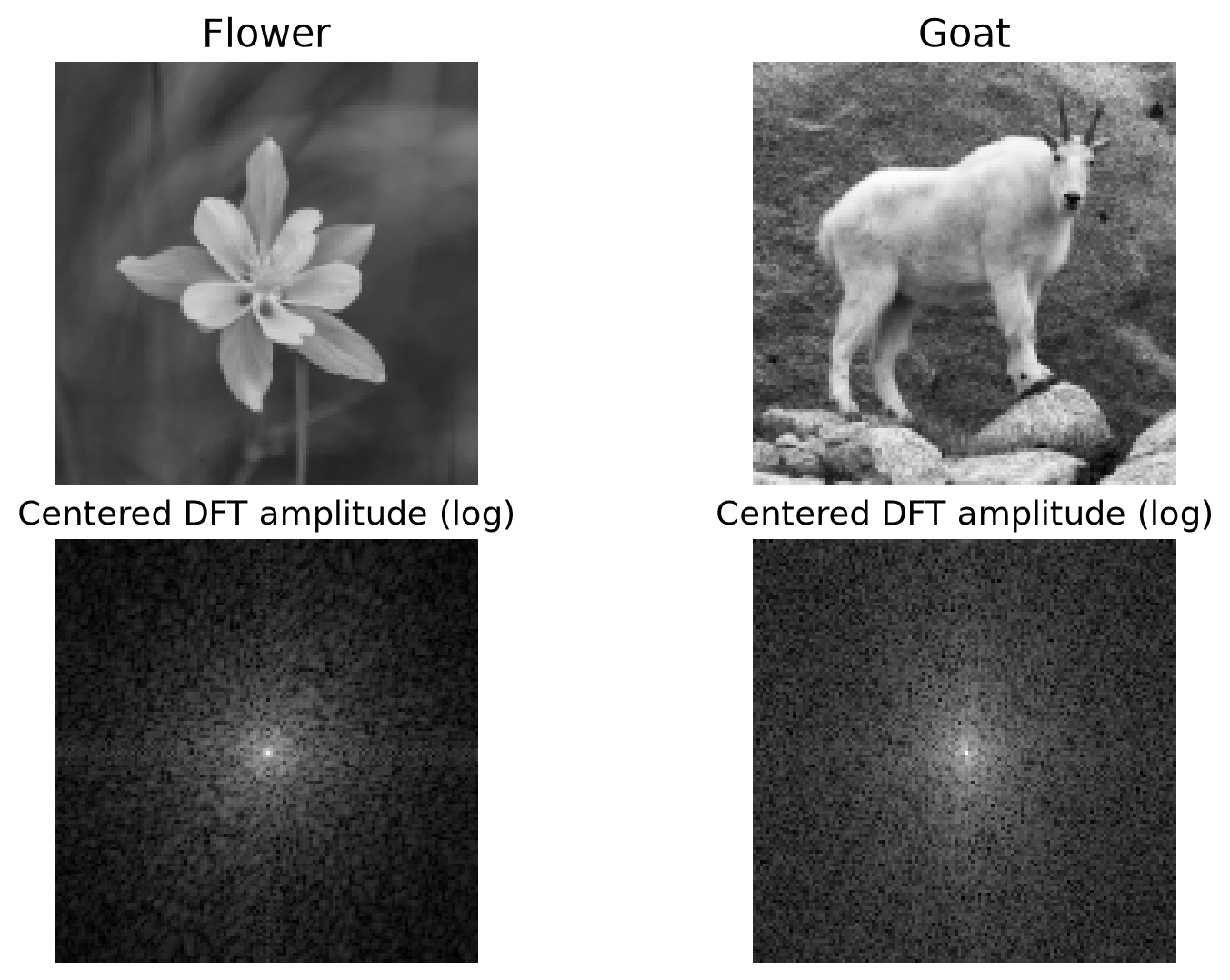
- In many natural images, large amplitudes concentrate near the center, at low spatial frequencies.
- Neighboring pixels often have similar intensities; edges and fine textures contribute higher frequencies.
What If Neighboring Pixels Are Unrelated?
Each pixel is drawn independently from a uniform distribution between \(0\) and \(1\).
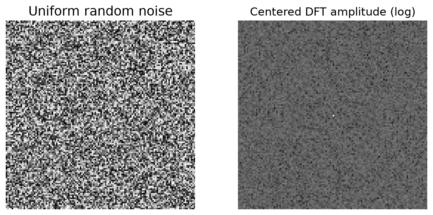
- Energy is spread broadly across frequencies, without a strong low-frequency concentration.
- The bright center point is because the image has a nonzero mean.
Keeping only low frequencies captures natural-image structure much better than random pixel detail.
Which Frequencies Do We See Best?
Natural images often concentrate energy at low frequencies.
Are our eyes equally sensitive to all spatial frequencies?
Where do you see the stripes?
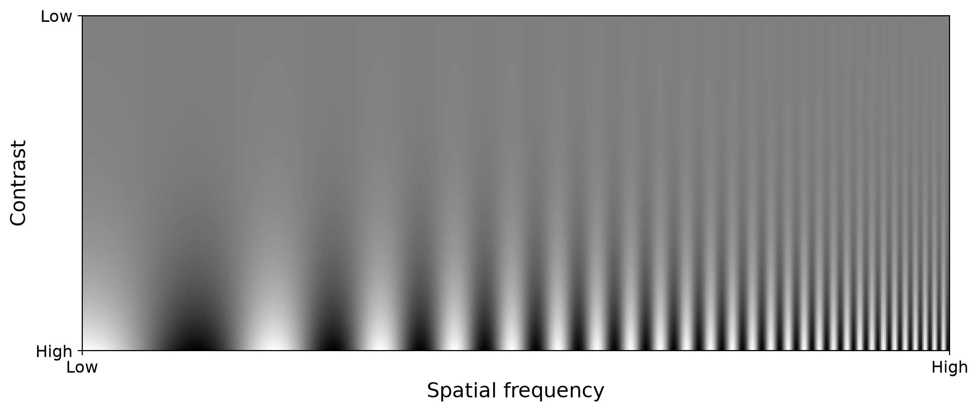
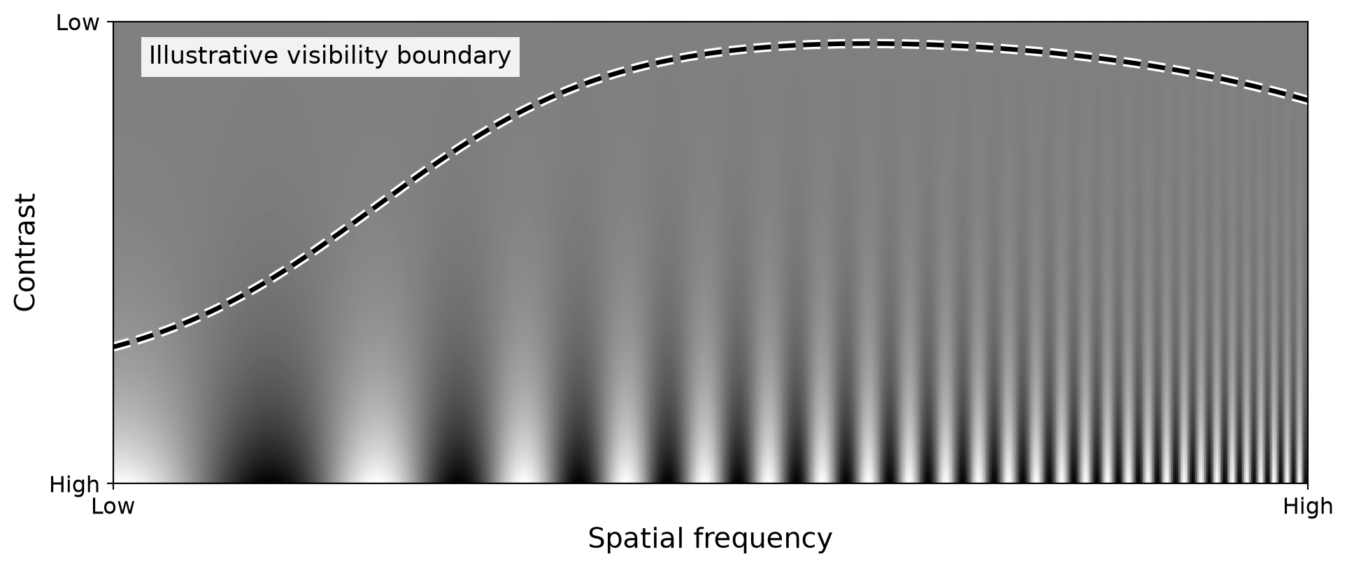
We typically detect lower contrast at intermediate spatial frequencies than at very low or very high frequencies.
Note: The curve illustrates the trend. Actual visibility depends on viewing distance, lighting, and the display.
The Same Filter in Two Domains
\[ y=\operatorname{corr}(I,h) \qquad \Longleftrightarrow \qquad Y=F\overline{H} \]
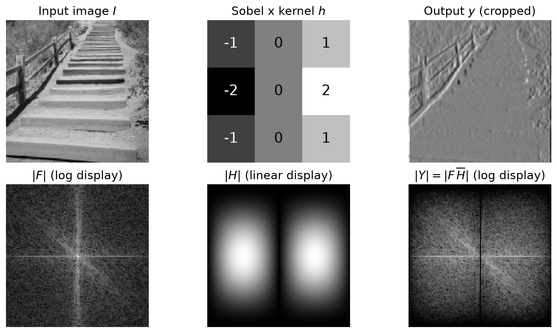
The Sobel x filter suppresses constant regions and responds to horizontal intensity changes, emphasizing vertical edges.
Revisiting Blurring: Box vs. Gaussian
Both filters average neighboring pixels. Why do their results look different?
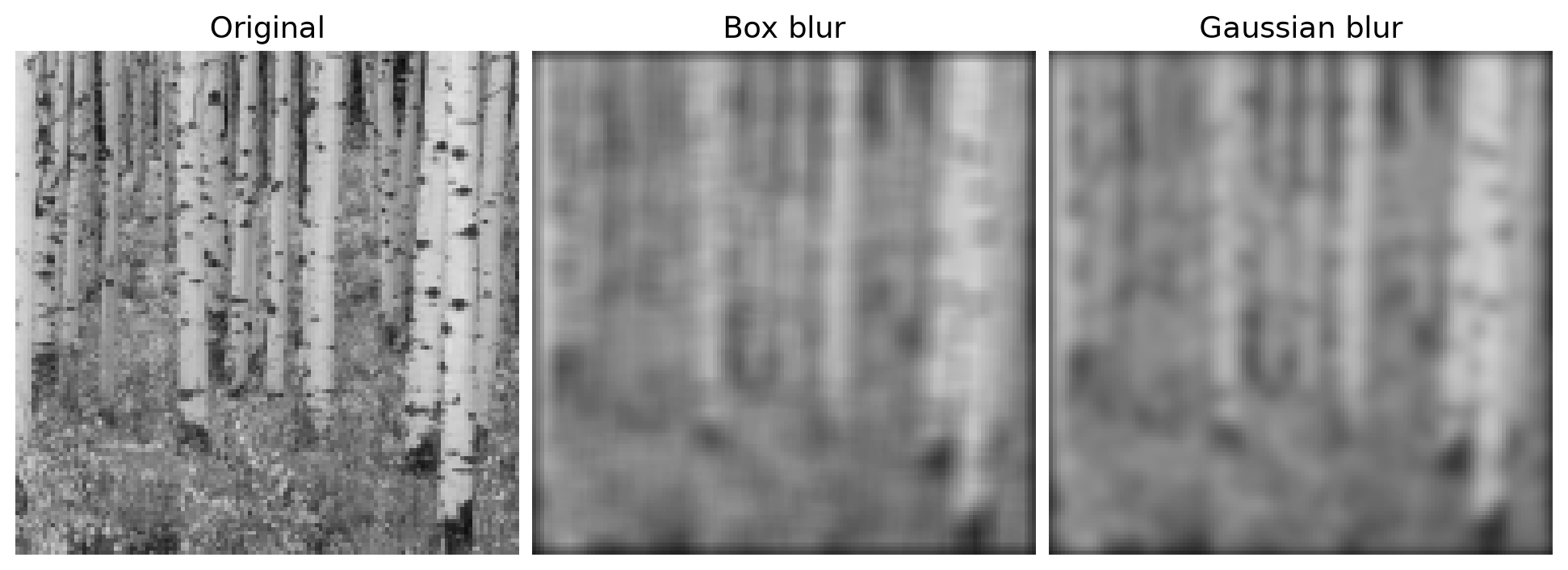
- Box: all pixels inside the window receive equal weight.
- Gaussian: weights decrease smoothly with distance from the center.
Their Fourier transforms reveal which frequencies each filter preserves or suppresses.
Gaussian Blur in the Frequency Domain
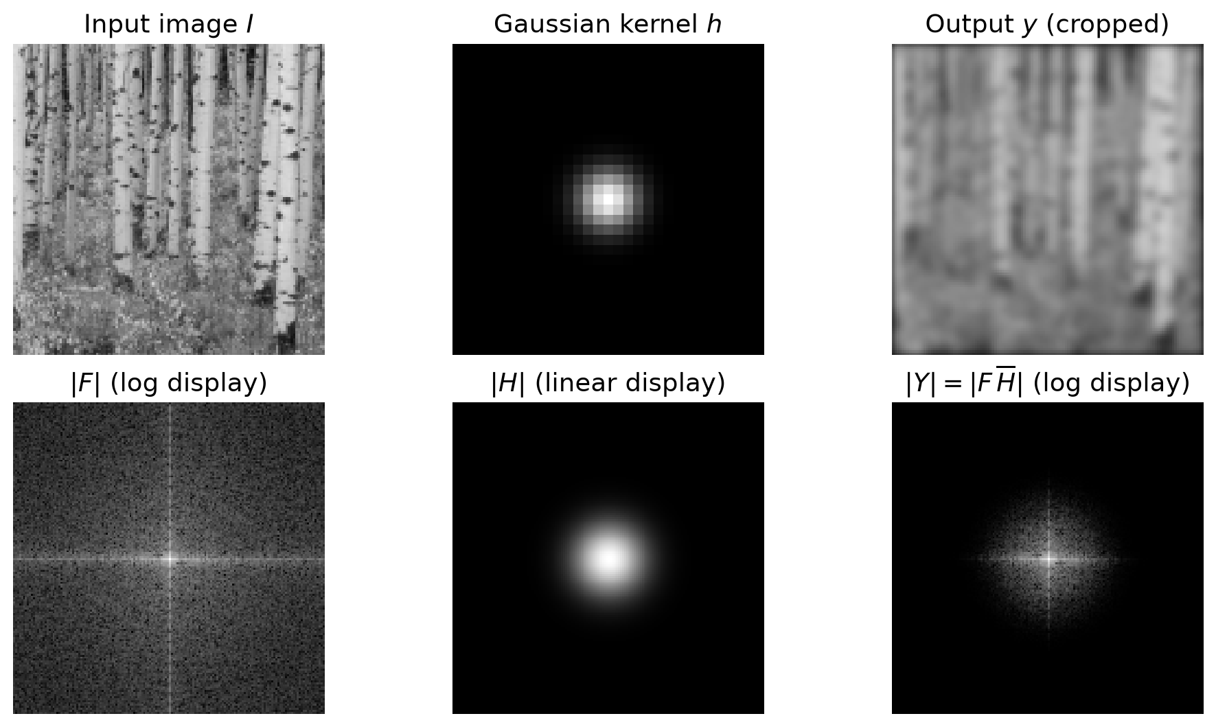
- The frequency response is Gaussian-shaped.
- Low frequencies pass through; higher frequencies are progressively attenuated.
Box Blur in the Frequency Domain
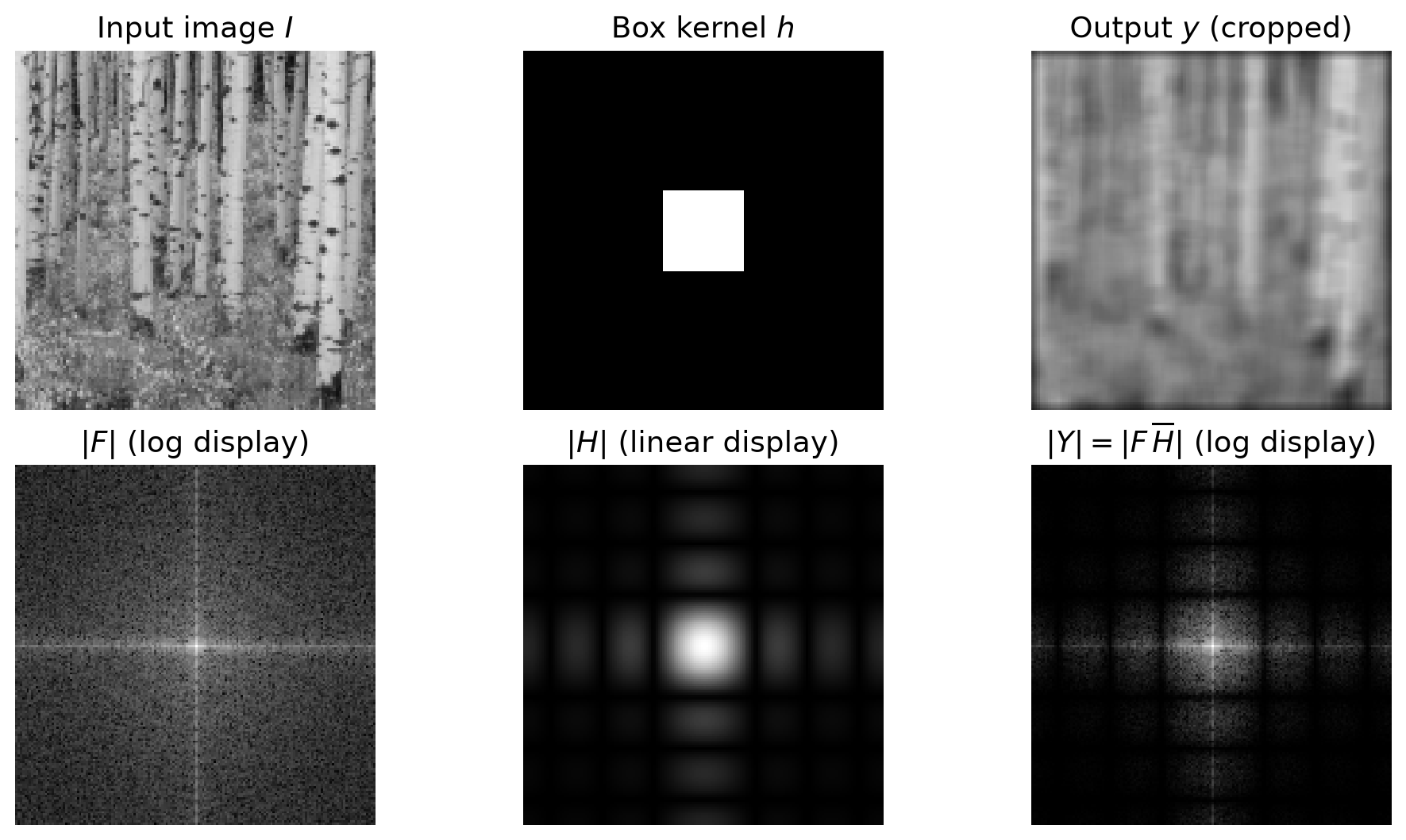
- The square kernel produces a sinc-like response with zeros and side lobes.
- Some frequency bands are suppressed strongly, while neighboring bands pass through more.
- This less uniform attenuation can leave more visible directional or block-like structure.
Quiz: Match Each Filter to Its Output
Match frequency-domain filters A–D to output images 1–4.
White passes frequencies; black removes them.
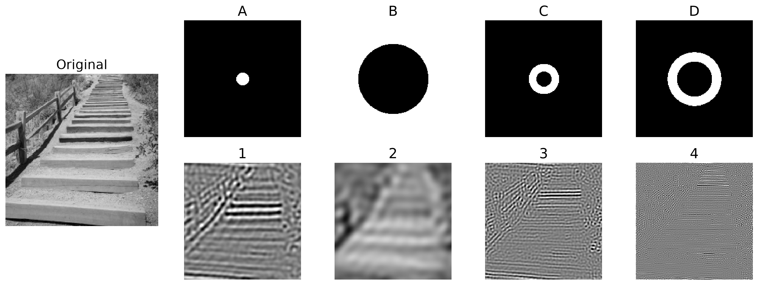
Which filters retain broad structures, intermediate details, or the finest texture?
Low-Pass Filtering Before Downsampling
Downsampling by 4 lowers the frequency limit to \(1/8\) cycle per original pixel in each direction.
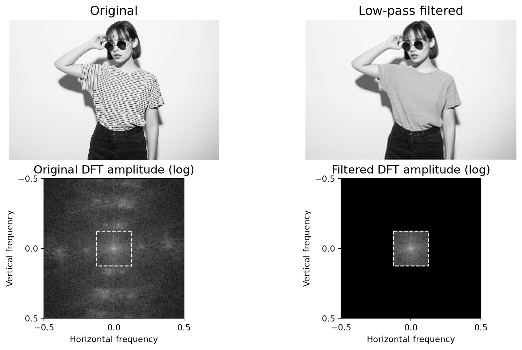
- The dashed box marks the frequencies the smaller image can represent.
- We remove frequencies outside that region before discarding pixels.
What Happens If We Skip the Filter?
Both downsampled images keep every fourth row and column.
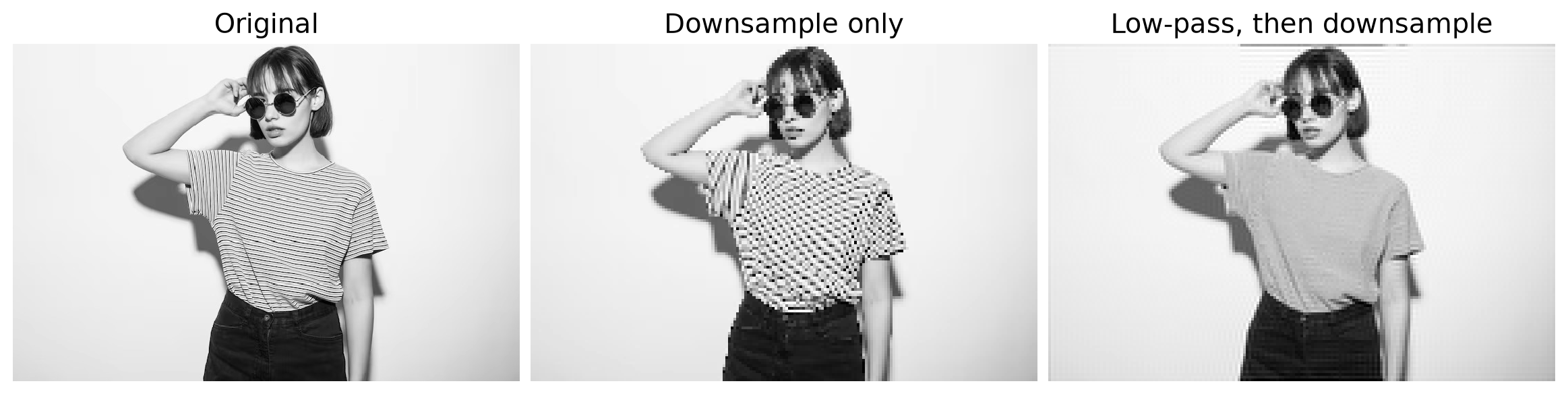
- Without filtering: fine stripes can become false coarse patterns—aliasing.
- With filtering: fine detail is deliberately removed before it can fold into lower frequencies.
Losing detail is preferable to inventing a different pattern.