Lecture 08 — Hough Transform
Lecture 8
From Edge Pixels to Lines
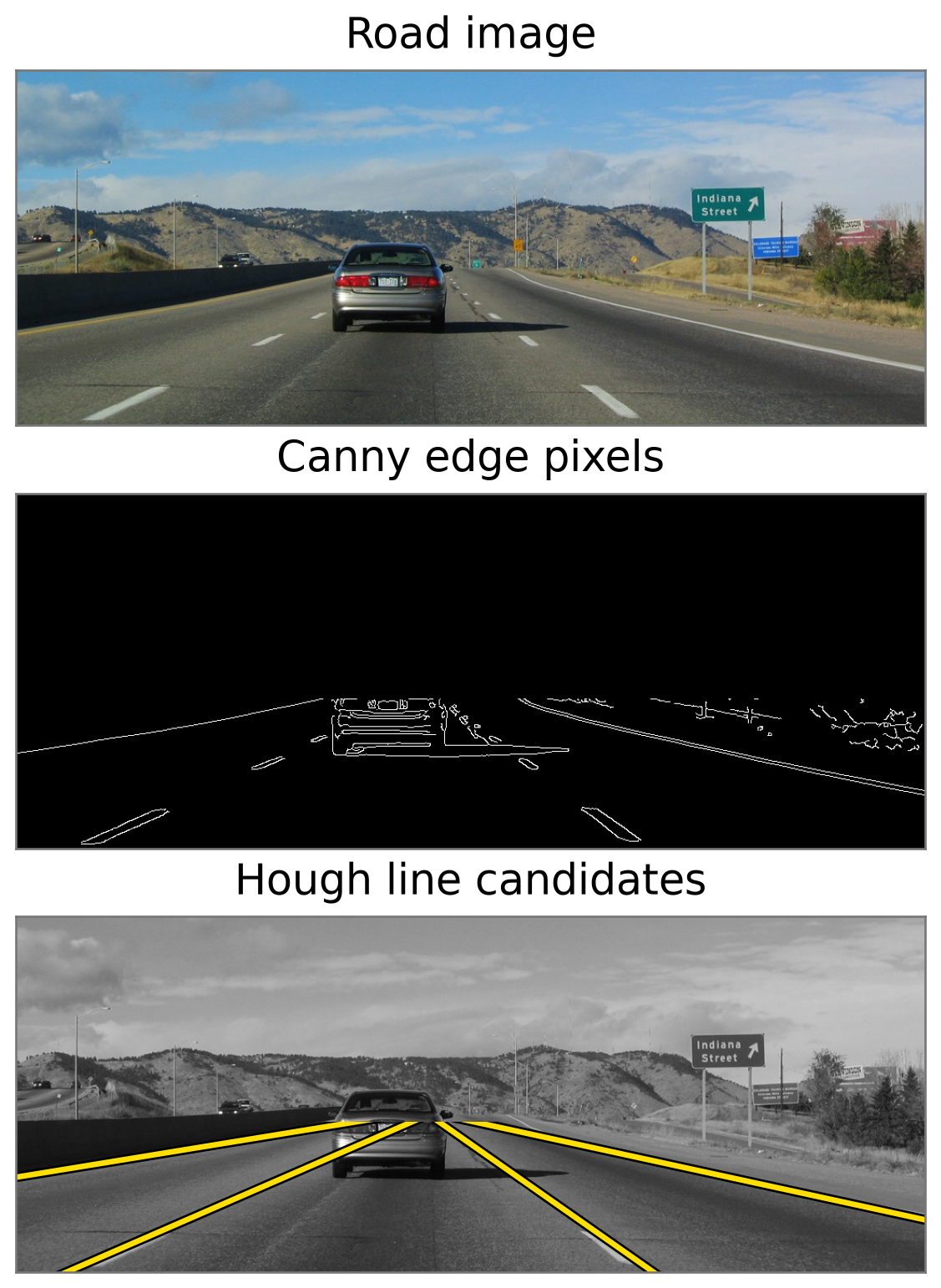
- Canny finds edge pixels at local intensity changes. It does not assign them to a shared line model.
- Hough groups supporting pixels into line models, including pixels separated by gaps.
- The yellow lines show four distinct candidates after excluding near-horizontal lines. Hough detects straight structures; it does not know which ones are lane boundaries.
Gaps Do Not Necessarily Prevent Detection
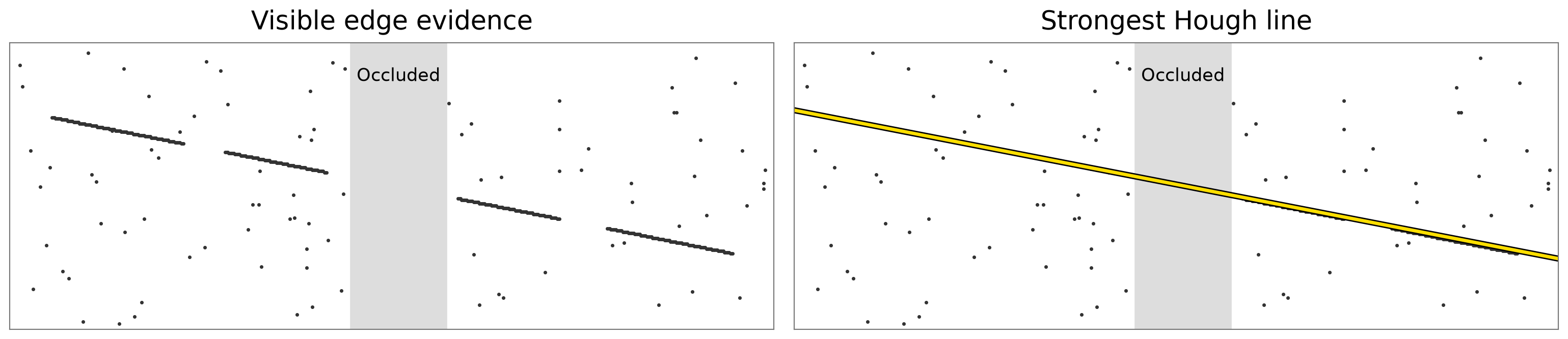
- Separated fragments can support the same line even when part of it is hidden.
- The detected line extends through the gap; this is a model prediction, not an observed edge.
- Detection still requires enough supporting evidence. Heavy clutter or too little visible structure can prevent a reliable result.
The Same Idea Can Detect Circles
A circle is a parametric model with center \((a,b)\) and radius \(r\):
\[ (x-a)^2 + (y-b)^2 = r^2 \]
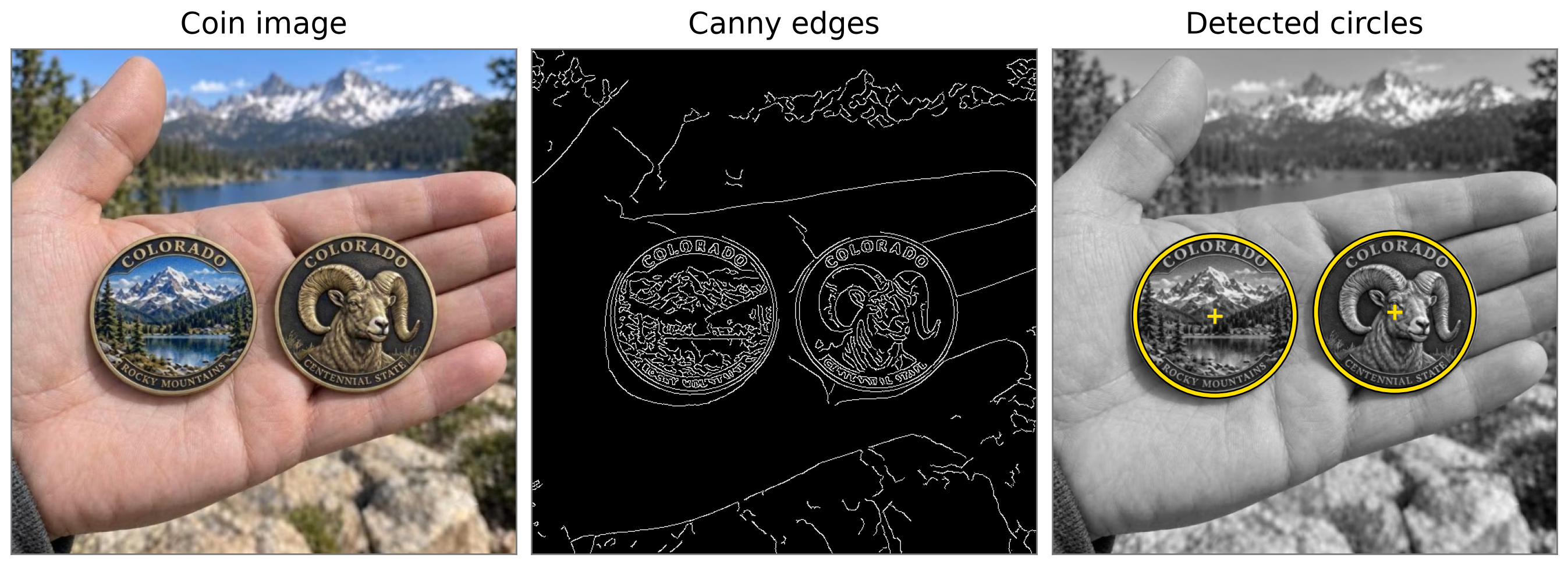
- Boundary evidence supports candidate circle centers and radii.
Representing a Line with Two Numbers
A line can be written as
\[ y = mx + b, \]
where \(m\) is its slope and \(b\) is its \(y\)-intercept.
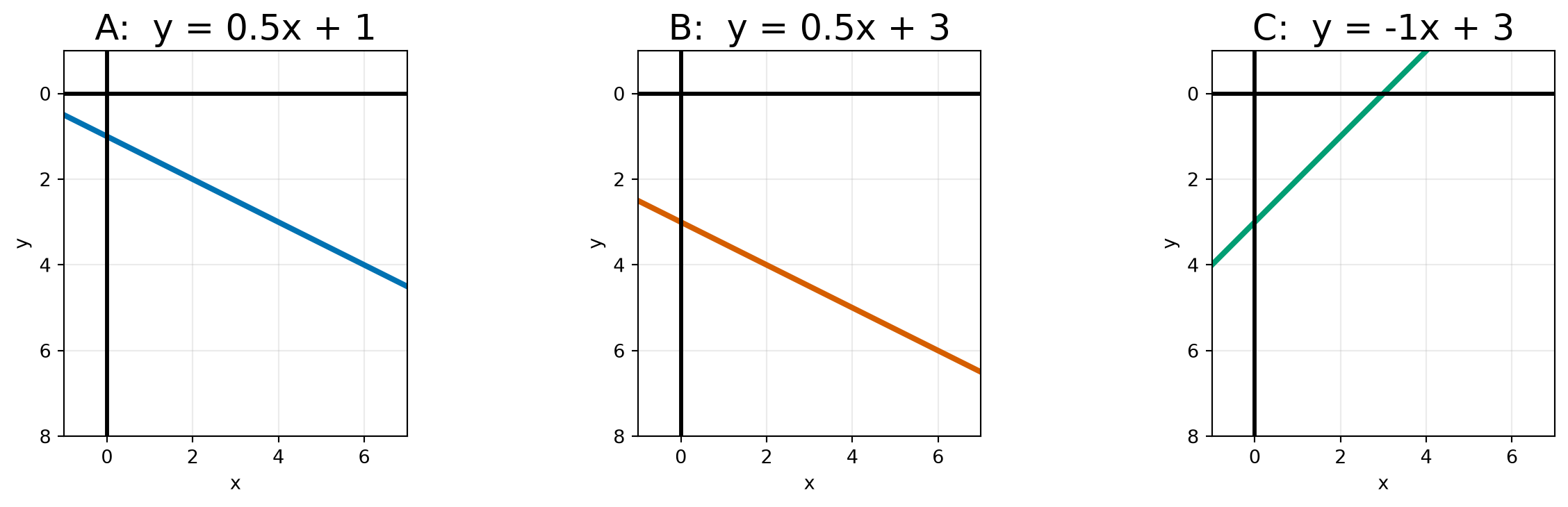
- Lines A and B have the same slope but different intercepts.
- Lines B and C have the same intercepts but different slopes.
A Line Becomes a Point
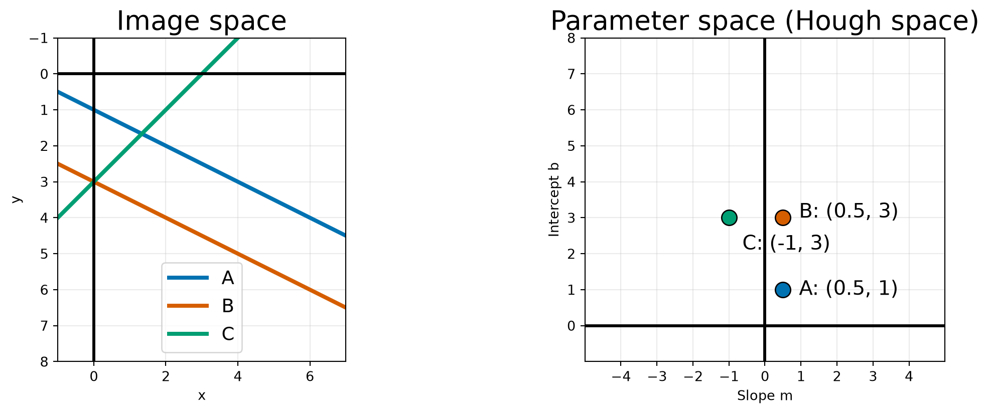
- In image space, a line has the equation \(y = mx + b\).
- In parameter space, a point specifies an entire line \((m,b)\).
- Parallel lines share the same \(m\) coordinate but have different \(b\) coordinates.
- Lines with the same intercept share the same \(b\) coordinate but can have different \(m\) coordinates.
Estimating a Line from an Edge Point
Given a point \((x,y)\) on an image edge that we want to estimate its line parameters:
- The image gradient \((I_x,I_y)\) is perpendicular to the edge.
- We can estimate its line parameters as: \[ m=-\frac{I_x}{I_y}, \qquad b=y-mx. \]
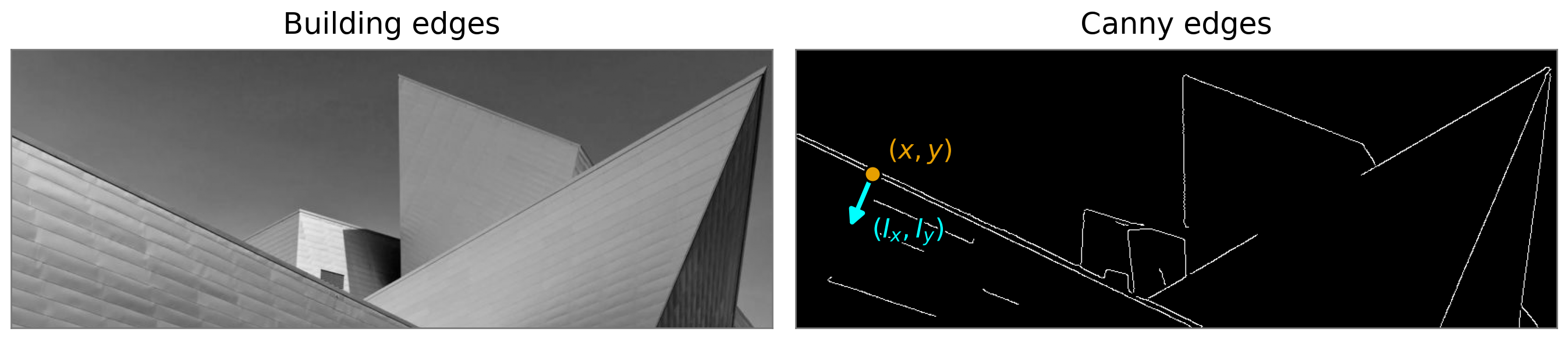
Each edge point now supplies an estimated line \((m,b)\) that we can count.
Note that near-vertical edges have \(I_y \approx 0\) and require a different representation, which we will address later.
Binning the Line Parameters
The parameters \(m\) and \(b\) are continuous. Divide their ranges into a grid of bins.
Voting in the Hough Space
- Initialize every bin to zero.
- Estimate \((m,b)\) at an edge point.
- Add one to the bin containing that estimate.
- Repeat for the other edge points.
- Nearby estimates can fall into the same bin.
- A bin’s value counts points that support a line model, not the number of separate physical lines.
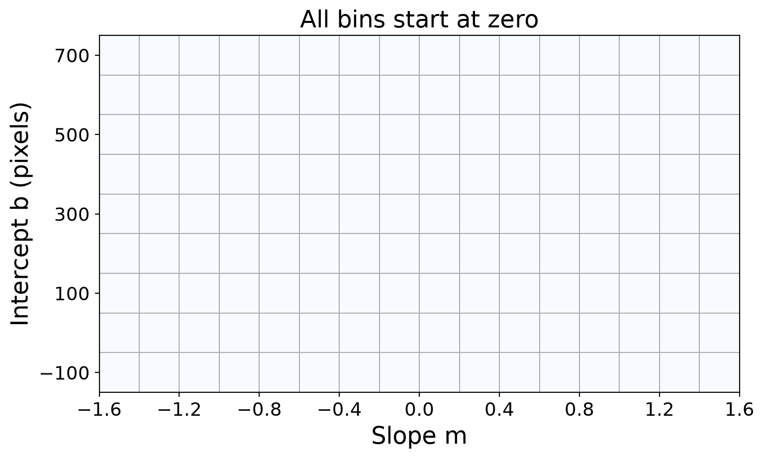
Each bin spans \(\Delta m=0.2\) and \(\Delta b=100\) pixels in this example.
One Edge Point, One Vote
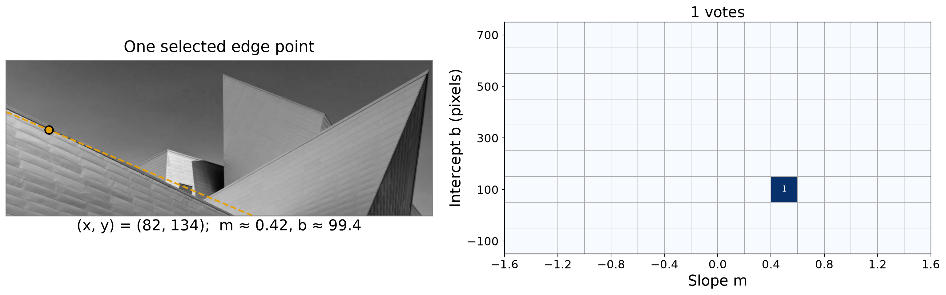
- The marked point and its gradient give one estimated line.
- That estimate falls into one parameter-space bin.
- We increment that bin by one.
More Points Add Votes
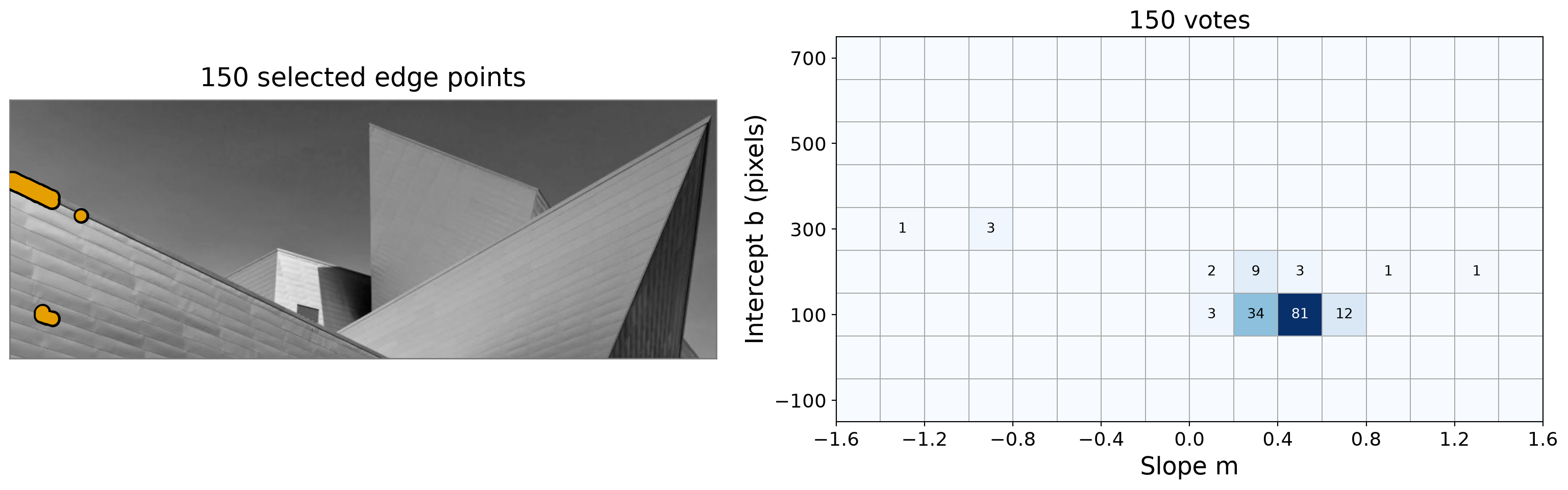
- Points along the same straight edge tend to produce similar slopes and intercepts.
- Their votes accumulate in the same bin or nearby bins.
- Noise, corners, and other edges spread votes across additional bins.
- A large count indicates strong support for a line with that bin’s parameters.
Peaks Identify Line Candidates
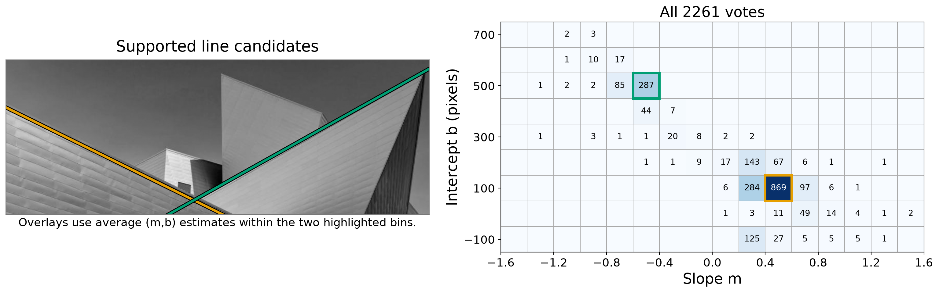
- Strong, separated peaks identify candidate lines supported by many edge points.
- Nearby bins may describe the same line, so we can suppress neighboring peaks.
- A high bin count measures support; it does not guarantee a correct detection.
Do We Need a Slope at Every Edge Point?
So far, each point must provide a unique line estimate:
\[ m=-\frac{I_x}{I_y}, \qquad b=y-mx. \]
- This requires a reliable gradient estimate.
- Noise and corners can make direction uncertain.
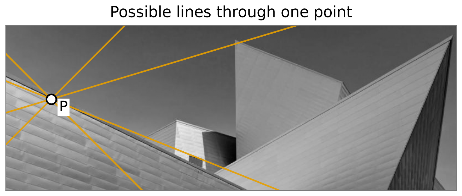
Can the point vote without first choosing one slope and intercept?
- Hough’s key idea: Instead of choosing one line from the gradient, let the point vote for all lines that could pass through it.
Which Lines Pass Through One Point?
For image point \(p = (2,3)\), any line through it must satisfy
\[ 3=2m+b \qquad\Longrightarrow\qquad b=3-2m. \]

- Choosing a slope \(m\), gives an intercept \(b\).
- Each possible image line contributes one parameter point. As we add more possibilities, those parameter points trace a line in Hough space.
Image Point Becomes a Hough Line
For a fixed image point \((x_0,y_0)\),
\[ y_0=mx_0+b \qquad\Longrightarrow\qquad \boxed{b=-x_0m+y_0.} \]
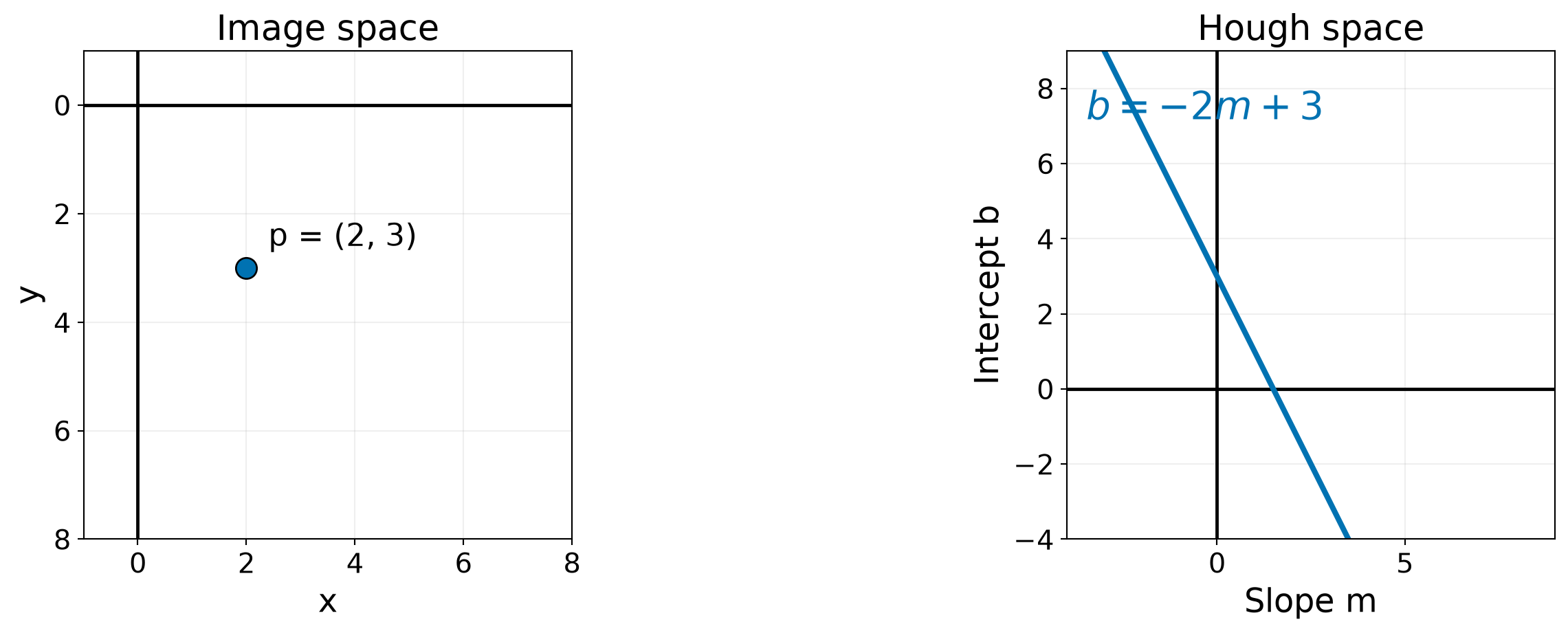
- In image space, \(x_0\) and \(y_0\) are fixed: we have one point.
- In Hough space, \(m\) and \(b\) vary: we have all possible lines through that point.
- The Hough-space line has slope \(-x_0\) and intercept \(y_0\).
Collinear Points Share an Intersection
Add points from the image line \(y=0.5x+2\). Each point contributes its own Hough-space line.

- Every blue Hough-space line passes through \((m,b)=(0.5,2)\).
- That shared intersection identifies the line containing all seven image points.
- Each additional collinear point adds support at the same parameters.
A Point Outside the Line
Now add \(q=(0,7)\), which does not lie on \(y=0.5x+2\). Its Hough-space line is \(b=7\).
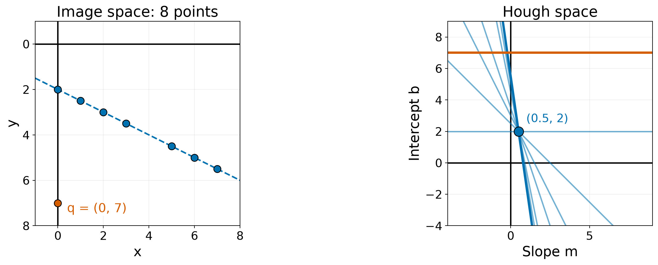
- The orange Hough-space line does not pass through the blue intersection.
- At \(m=0.5\), it gives \(b=7\), rather than \(b=2\).
- It crosses individual blue lines elsewhere, but those pairwise intersections have less support.
Another Group Produces Another Intersection
Add more points collinear with \(q\), along \(y=5x+7\).

- The blue group supports \((m,b)=(0.5,2)\).
- The orange group supports \((m,b)=(5,7)\).
- Multiple image lines produce multiple locations where many Hough-space lines intersect.
- The colors distinguish the known groups in this example. In an image, we must discover the groups from their votes.
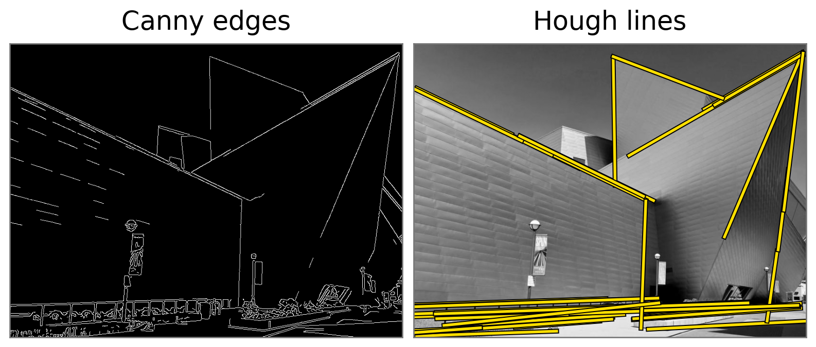
Detecting the Museum Lines Without Edge Directions
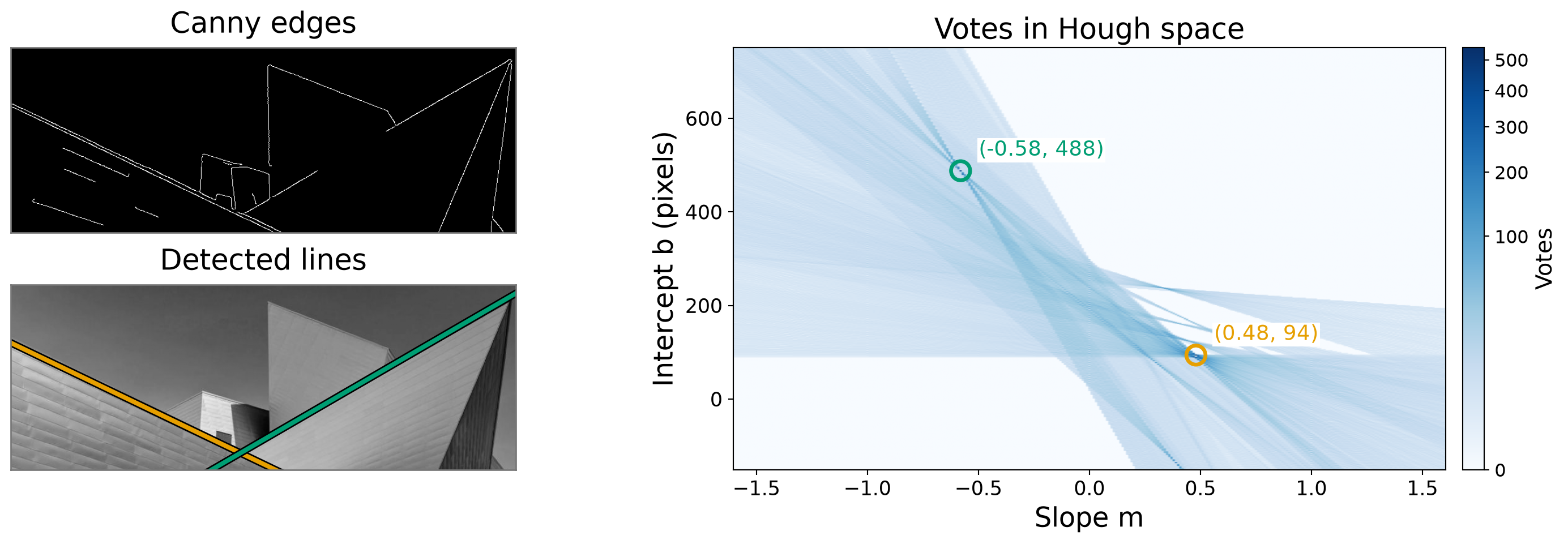
- Many Hough-space lines overlap near each detected peak.
- The peaks recover the two main building edges.
- Voting uses edge locations only; it does not use their gradient directions.
What Happens to a Vertical Line?
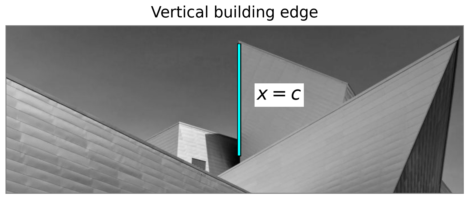
The highlighted, nearly vertical building edge is modeled as \(x=c\).
What is its slope?
- An exactly vertical line has an undefined slope.
- No finite pair \((m,b)\) represents it as \(y=mx+b\).
How large must Hough space be?
For lines through \((x_0,y_0)\),
\[ b=y_0-m x_0. \]
When \(x_0>0\),
\[ m\rightarrow+\infty \quad\Longrightarrow\quad b\rightarrow-\infty. \]
How can we represent all line orientations without unbounded slopes and intercepts?
Representing a Line with Distance and Angle
Instead of slope and intercept \((m,b)\), describe a line using \((r,\theta)\):
- \(\theta\) is the angle of the line’s normal, measured from the positive \(x\) axis in the range \(0\leq\theta<180^\circ\).
- \(r\) is the signed perpendicular distance from the origin. The geometric distance is \(|r|\).
Given image gradient \((I_x, I_y)\) or line equation \(y = mx + b\):
- \(\theta = \operatorname{atan2}(I_y, I_x) \bmod \pi\), or \(\theta = \operatorname{atan2}(1,-m)\).
- \(r = x\cos\theta+y\sin\theta\) for any point \((x,y)\) on the line, or \(r = \frac{b}{\sqrt{m^2+1}}\).
- If \(r>0\), the closest point on the line lies along the chosen normal from the origin.
- If \(r<0\), it lies in the opposite direction.
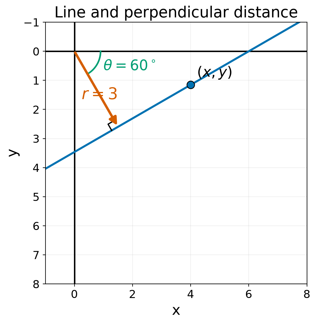
We keep image coordinates: \(x\) points right and \(y\) points down, so positive \(\theta\) appears clockwise.
Binning the Polar Parameters
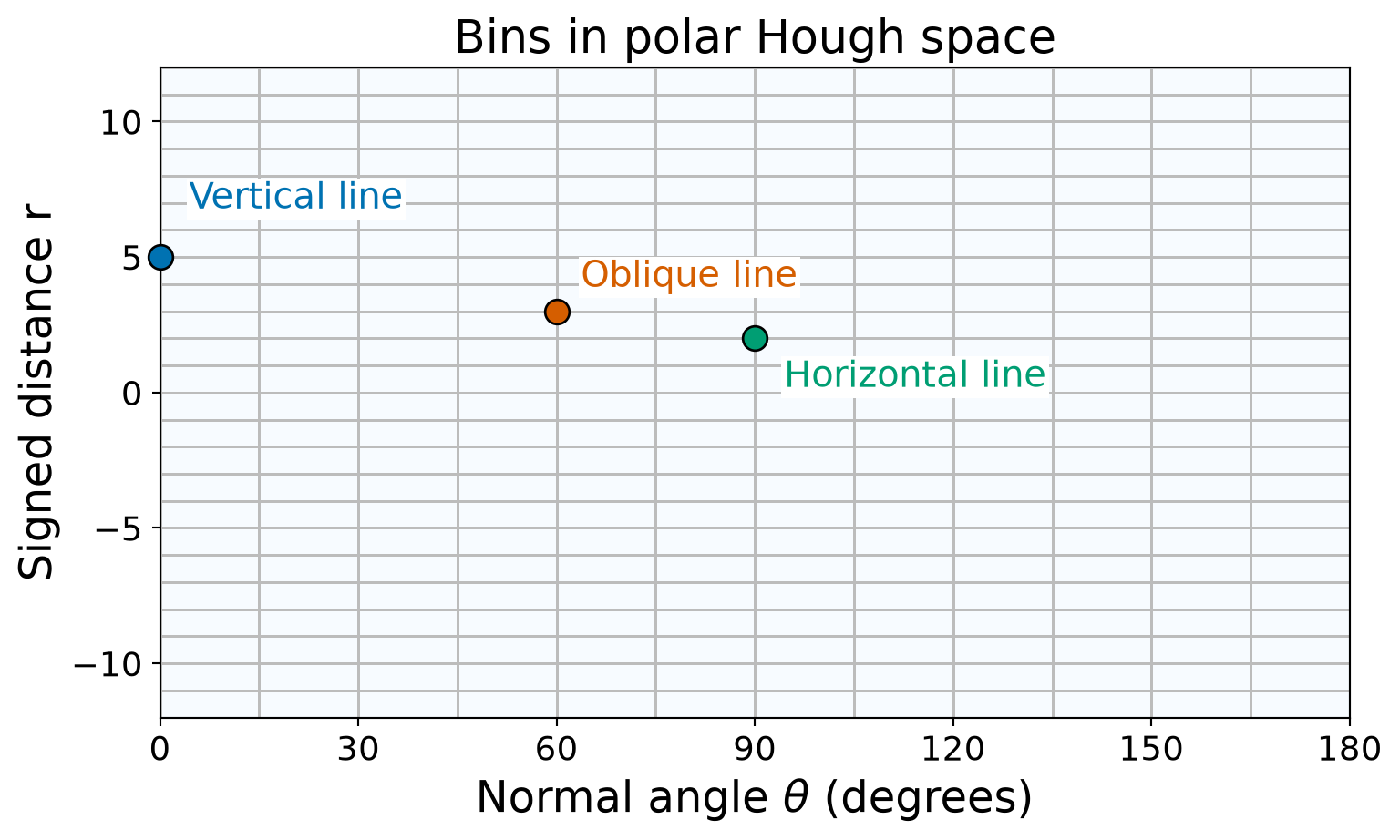
- Divide Hough space into angle and distance bins.
- Use \(0\leq\theta<180^\circ\), and \(-D\leq r\leq D\).
- For a \(W\times H\) image, \(D=\sqrt{(W-1)^2+(H-1)^2}\).
- A vertical line \(x=c\) has \(\theta=0^\circ\) and \(r=c\).
- A horizontal line \(y=c\) has \(\theta=90^\circ\) and \(r=c\).
- All orientations now have finite parameters.
Polar Hough Voting
- For each edge point \((x,y)\), try each sampled angle \(\theta\).
- Compute \(r=x\cos\theta+y\sin\theta\) and increment the corresponding bin.
- Find strong peaks to identify supported line models.
A Point Becomes a Sinusoid
For the same image point \(p=(2,3)\), the possible line parameters satisfy
\[ r(\theta)=2\cos\theta+3\sin\theta. \]

- Rotating the normal selects different lines through the same image point.
- Each candidate line gives one point in Hough space. Together, these points trace a sinusoid.
- The green arrow shows the normal direction. The dashed segment connects the origin to the closest point on the line.
Collinear Points Share a Polar Intersection
Use the same image points on \(y=0.5x+2\). Each point now contributes a sinusoid.

- All seven curves pass through the same parameters: \(\theta\approx116.6^\circ\), \(r\approx1.79\).
- These parameters describe the original image line.
- Additional collinear points reinforce the same Hough-space location.
What Changes When Points Are Noisy?
Add small position errors to points sampled from the same line \(y=0.5x+2\).
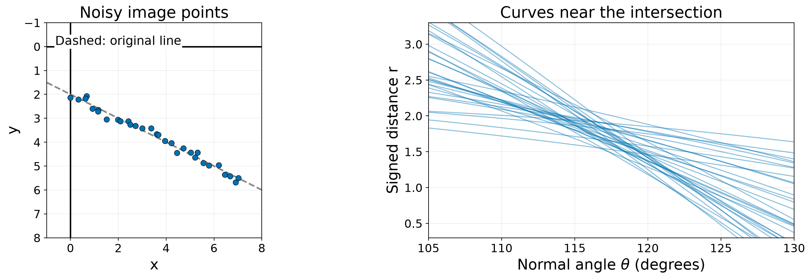
- The points no longer lie exactly on one line.
- Their sinusoids no longer share one exact intersection.
- Support spreads across a neighborhood in Hough space, so we look for a concentration of votes.
Bin Size and Noisy Votes
Use the same noisy points with two different accumulator grids.
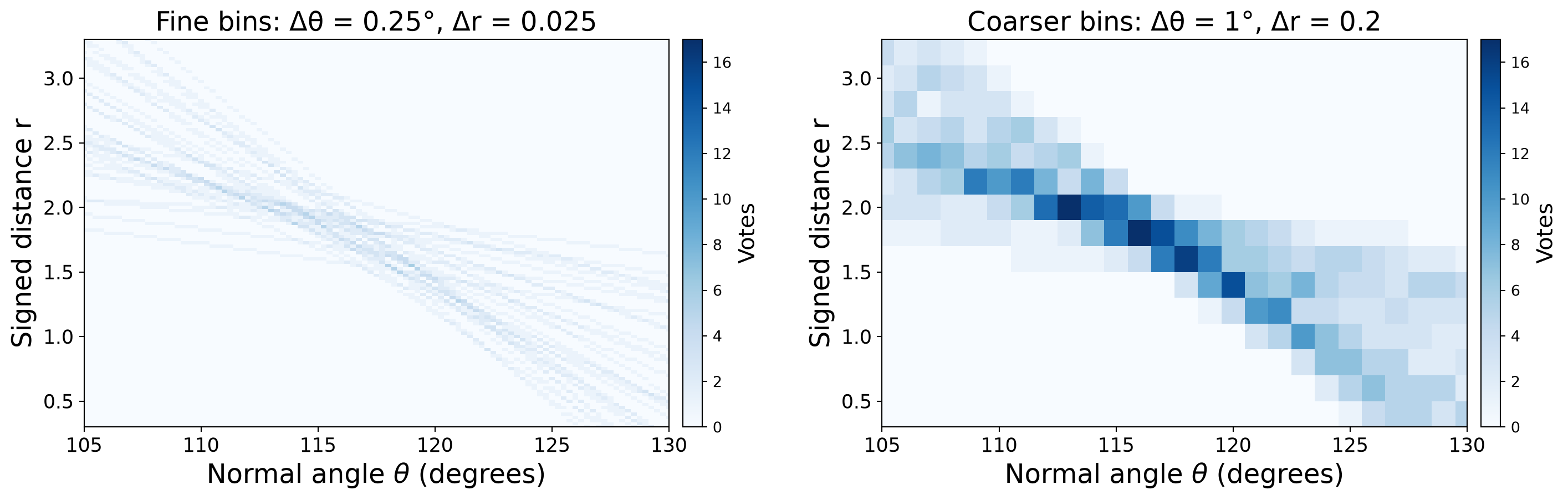
- Fine bins provide precise parameter locations, but noise can split support across many bins.
- Coarser bins collect more nearby votes, but reduce precision and can merge distinct lines.
- Lightly smoothing the accumulator can combine neighboring support before finding peaks.
- For multiple lines, suppress nearby peaks. To recover line segments, examine the supporting image points and their gaps.
Hough Line Detection in OpenCV
field_gray = cv2.cvtColor(field_rgb, cv2.COLOR_RGB2GRAY)
field_polygon = np.array([[310, 28], [1220, 120],
[1190, 400], [40, 160]], dtype=np.int32)
field_mask = np.zeros_like(field_gray)
cv2.fillPoly(field_mask, [field_polygon], 255)
field_smooth = cv2.GaussianBlur(field_gray, (5, 5), 1.2)
field_edges = cv2.Canny(field_smooth, 40, 100)
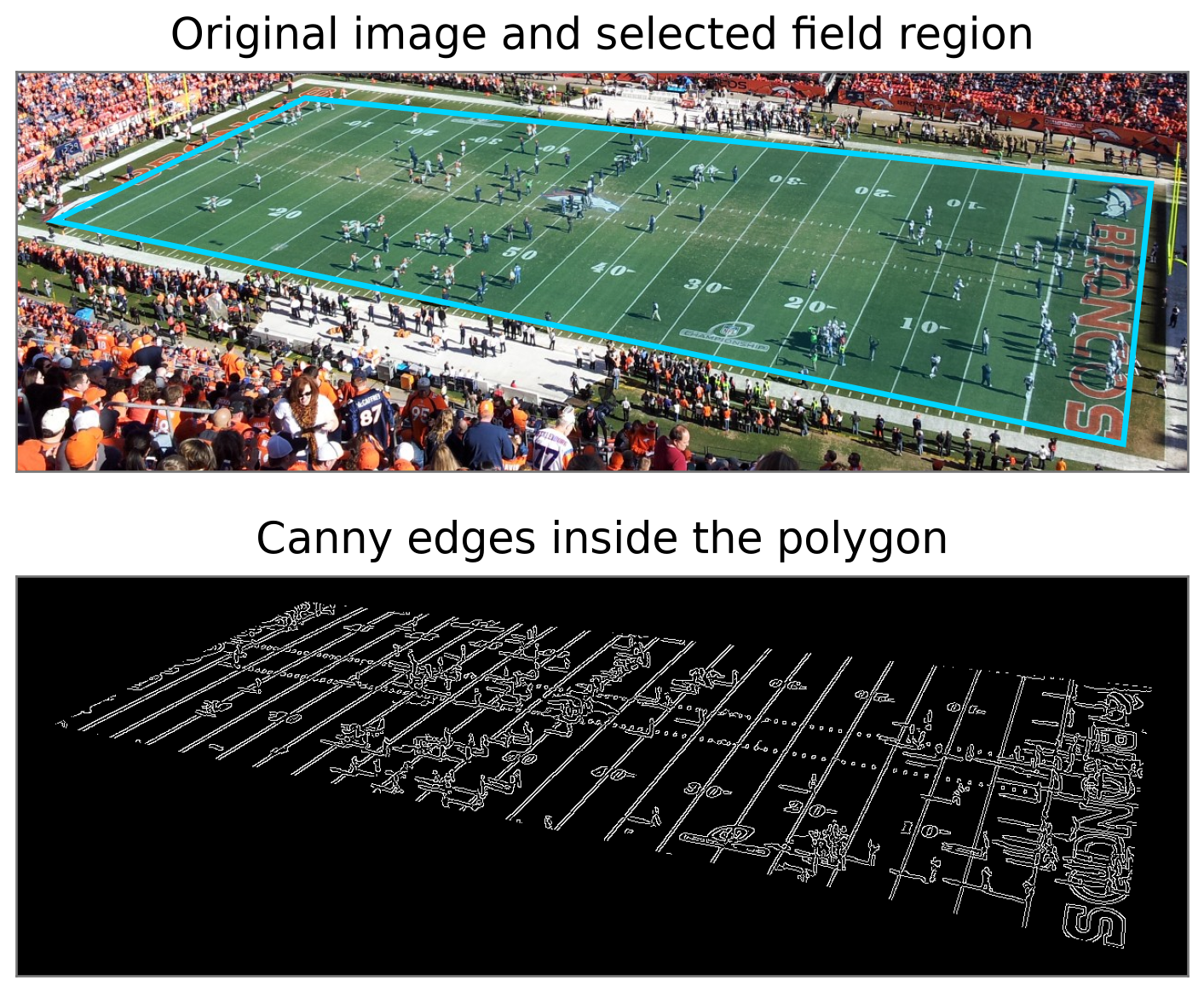
field_edges = cv2.bitwise_and(field_edges, field_mask)- Gaussian smoothing reduces noise & small intensity variations.
- Canny uses thresholds of 100 for strong edges and 40 to continue connected weaker edges.
- We apply a mask after Canny to search only for lines inside the field.
Hough Line Detection in OpenCV
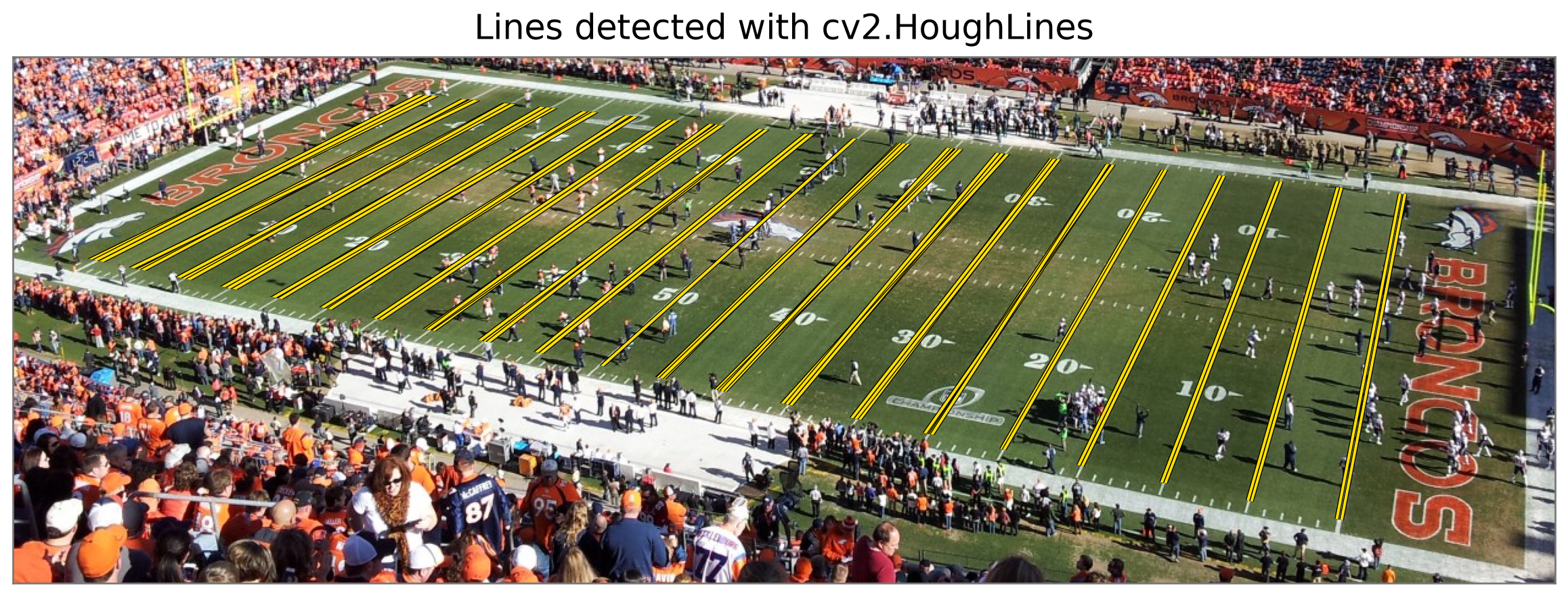
Each returned \((r,\theta)\) defines a line: \(x\cos\theta+y\sin\theta=r\).
rho=1: distance bins spaced 1 pixel apart.theta: angle bins spaced 1° apart, supplied in radians.threshold=140: a peak must exceed 140 votes. Lower values admit weaker lines and more false detections.min_theta,max_theta: search normal angles from 0° to 80°, targeting the yard lines in this image.
Circle Detection
A circle has center \((a,b)\) and radius \(r\):
\[ (x-a)^2+(y-b)^2=r^2. \]
If \(r\) is known, an edge point \((x,y)\) votes for all centers \((a,b)\) at distance \(r\) from it.
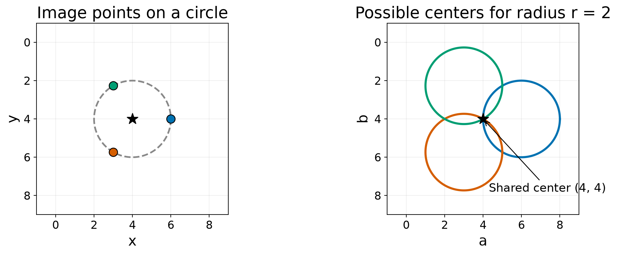
- Each colored point produces a circle of possible centers in the \((a,b)\) parameter space.
- Points on the same image circle support a shared center. Binning these votes produces a peak.
Searching for the Radius
When the radius is unknown, the full parameter space is three-dimensional: \((a,b,r)\).
- A direct approach repeats center voting for each tested radius.
- Gradient directions reduce the search: a circle’s normal passes through its center.
For a unit gradient direction \(\hat{\mathbf{g}}\) at an edge point,
\[ \begin{bmatrix}a\\b\end{bmatrix} = \begin{bmatrix}x\\y\end{bmatrix} \pm r\hat{\mathbf{g}}. \]
Gradient-Based Radii Search
- Find edges and their gradient directions.
- Vote for centers along those directions.
- Estimate radii supported by edges around each candidate center.
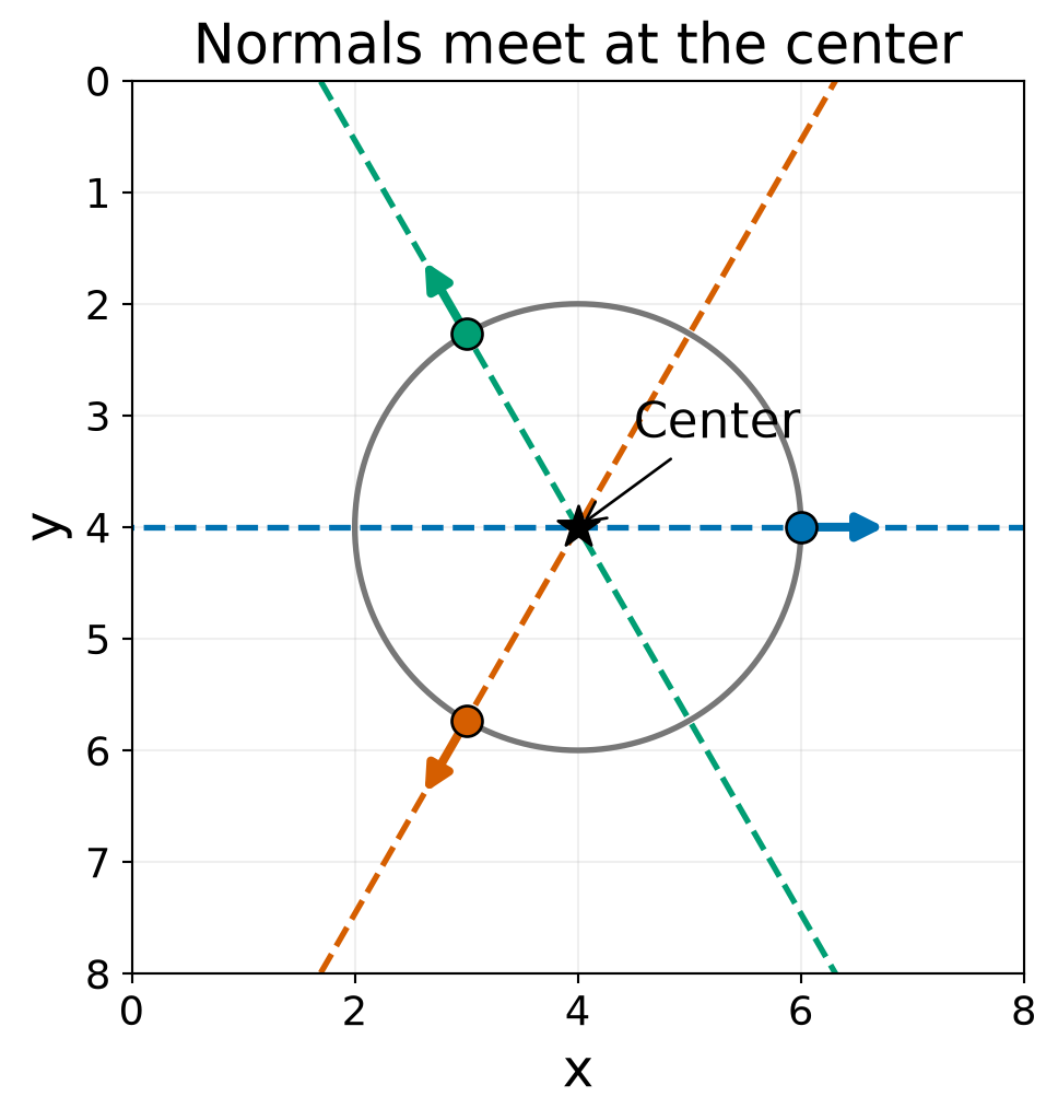
Ideal circle normals are shown here. Measured gradients are noisy, so nearby votes must be combined.
Hough Circle Detection in OpenCV
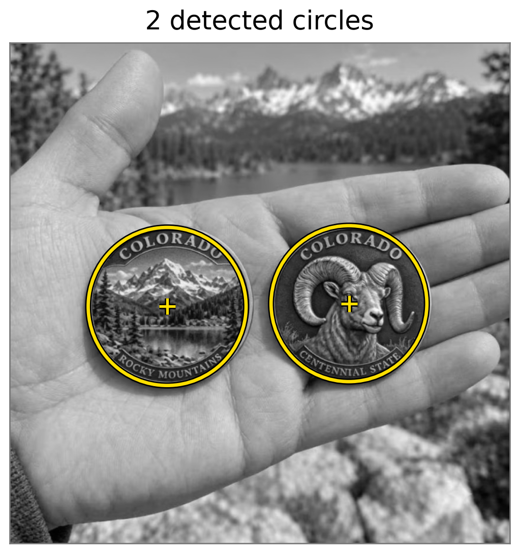
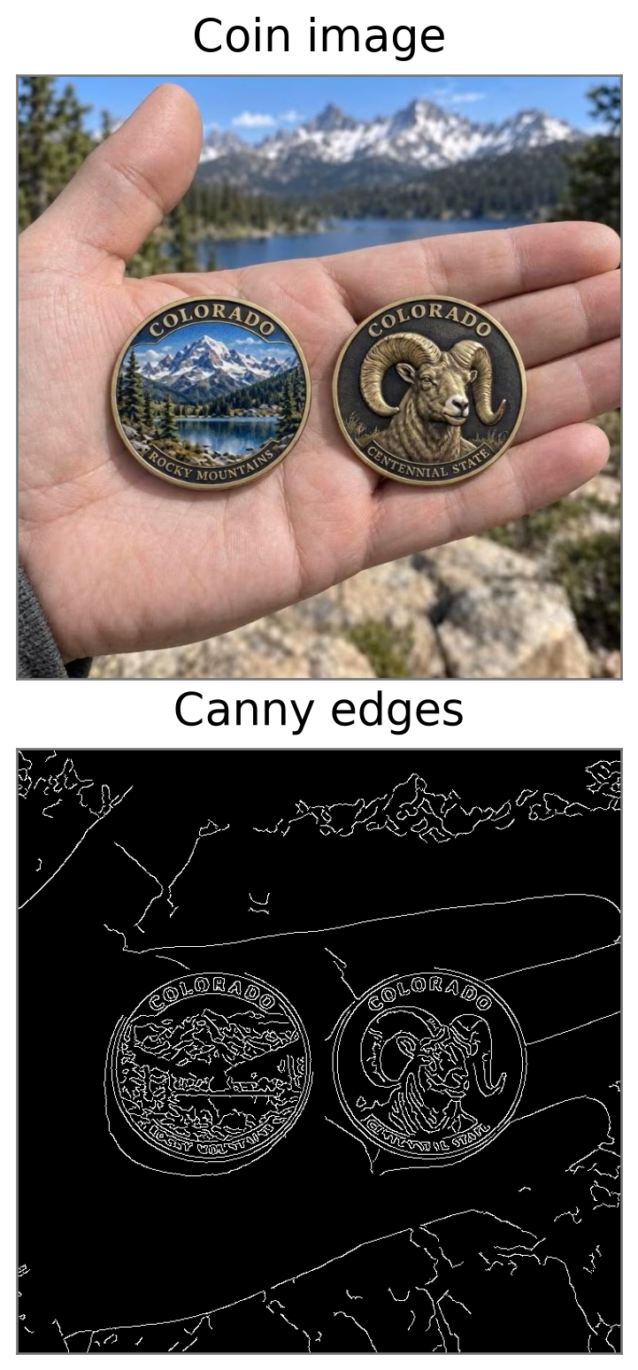
- Smoothing reduces noise & fine textures while preserving the coin outlines.
- Canny also detects lettering and background edges.
- We pass the smoothed grayscale image to
HoughCirclesto computes edges and gradients (internally). Cannyis for visualization only;HoughCirclescomputes edges internally.
Hough Circle Detection in OpenCV
dp=1.2: center-accumulator cells span approximately 1.2 image pixels.minDist=170: minimum separation between detected centers; reduces duplicate detections.param1=120: upper internal Canny threshold; the lower threshold is set to half of this value as 60.param2=45: voting threshold for accepting circle candidates. Lower values admit weaker candidates and more false detections.minRadius,maxRadius: search radii from 85 to 115 pixels in the image.
Each result contains \((a,b,r)\): center coordinates and radius.