Lecture 10 — Optical Flow

Lecture 10

Kaveh Fathian

Computer Science Department, Colorado School of Mines

Learning Objectives

By the end of this lecture, you should be able to:

  • Explain optical flow, distinguish sparse and dense estimates, and describe their applications.
  • Derive the optical flow constraint from brightness constancy and explain the aperture problem.
  • Explain how Lucas–Kanade estimates motion within a window, why corners are suitable for tracking, and how image pyramids help handle larger motion.
  • Use OpenCV to track selected points and estimate dense optical flow.

Fundamental Equations of Computer Vision

1. Image Filtering \(\displaystyle y[m,n]=\sum_{k,l} h[k,l]\,I[m+k,n+l]\)
2. Optical Flow \(\displaystyle I(x,y,t)=I(x+\Delta x,\ y+\Delta y,\ t+\Delta t)\)
3. Camera Geometry \(\displaystyle \mathbf{x}=\mathbf{K}\begin{bmatrix}\mathbf{R}&\mathbf{t}\end{bmatrix}\mathbf{X} \qquad \mathbf{x}^{T}\mathbf{F}\mathbf{x}'=0\)
4. Machine Learning \(\displaystyle \underset{\mathcal{S}}{\operatorname{arg\,min}}\sum_{i=1}^{k}\sum_{\mathbf{x}\in S_i}\left\lVert\mathbf{x}-\boldsymbol{\mu}_i\right\rVert^{2} \qquad y=\varphi\!\left(\mathbf{w}^{T}\mathbf{x}+b\right)\)

What Is Optical Flow?

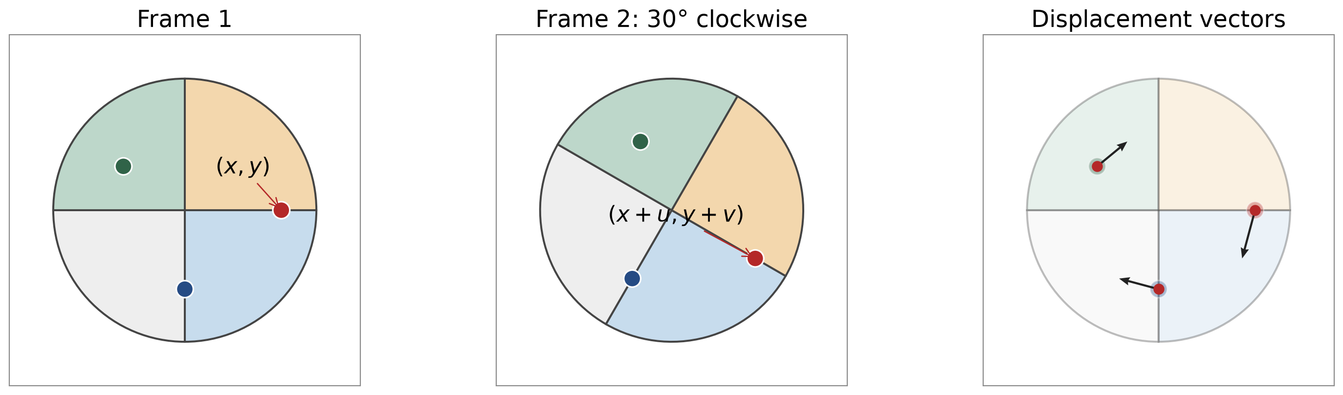
  • Optical flow describes the apparent motion of image points between video frames.

  • A point at \((x,y)\) moves to \((x+u,y+v)\), giving a displacement vector \((u,v)\).

Note: Image coordinates increase to the right and downward.

  • Motion can result from movement of the object, the camera, or both.
  • \((u,v)\) describes displacement in image pixels, not directly the object’s 3D motion.

Sparse and Dense Optical Flow

  • Sparse optical flow: estimated displacement at selected image points, often corners.
  • Dense optical flow: estimated displacement at every pixel.
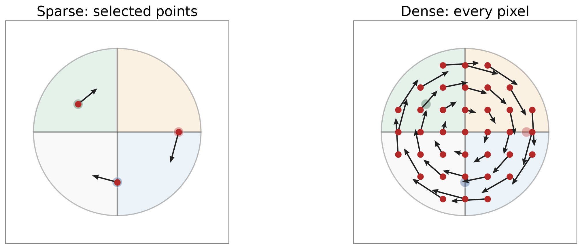
Only a subset of the dense field’s arrows is displayed for readability.

  • Sparse estimates are often used for tracking selected features.
  • Dense estimates describe motion across the image, including regions with different motions.

Visualizing Optical Flow

Optical flow is often displayed using arrows or colors.
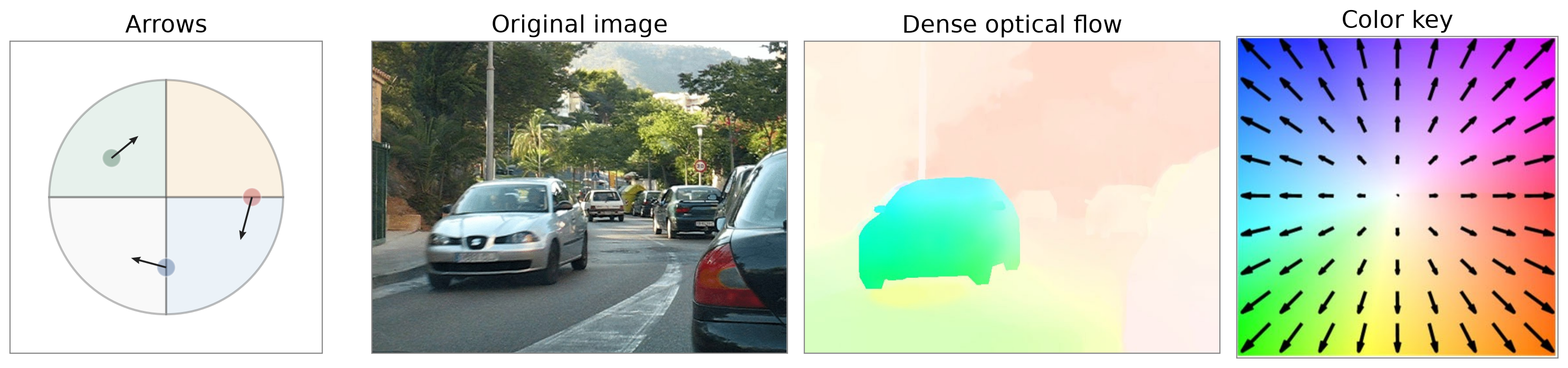
  • Arrows: direction indicates where a point moves; length represents displacement magnitude.
  • Colors: encode a dense field. E.g., hue represents direction; stronger color away from white represents larger displacement.

Optical Flow Applications

Optical Computer Mouse
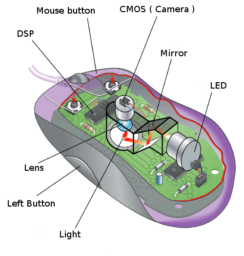
jason@heqingele.com; pexels
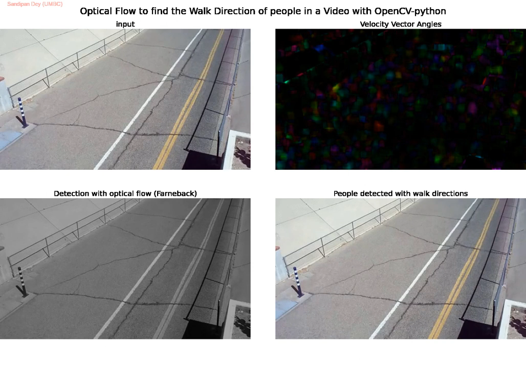
Pedestrian Detection
& Motion Estimation

Watch on YouTube

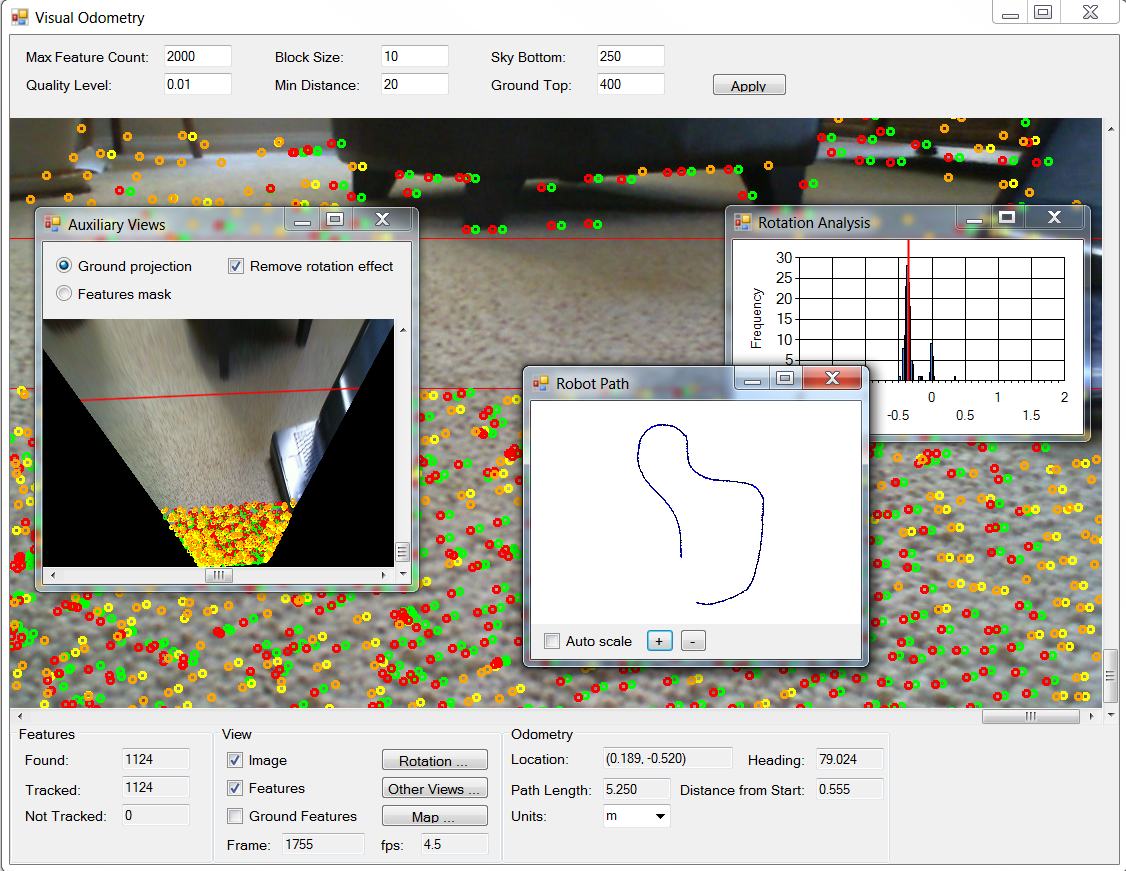
Visual Odometry & SLAM

Rainer Hessmer

Optical Flow Applications

Super Resolution
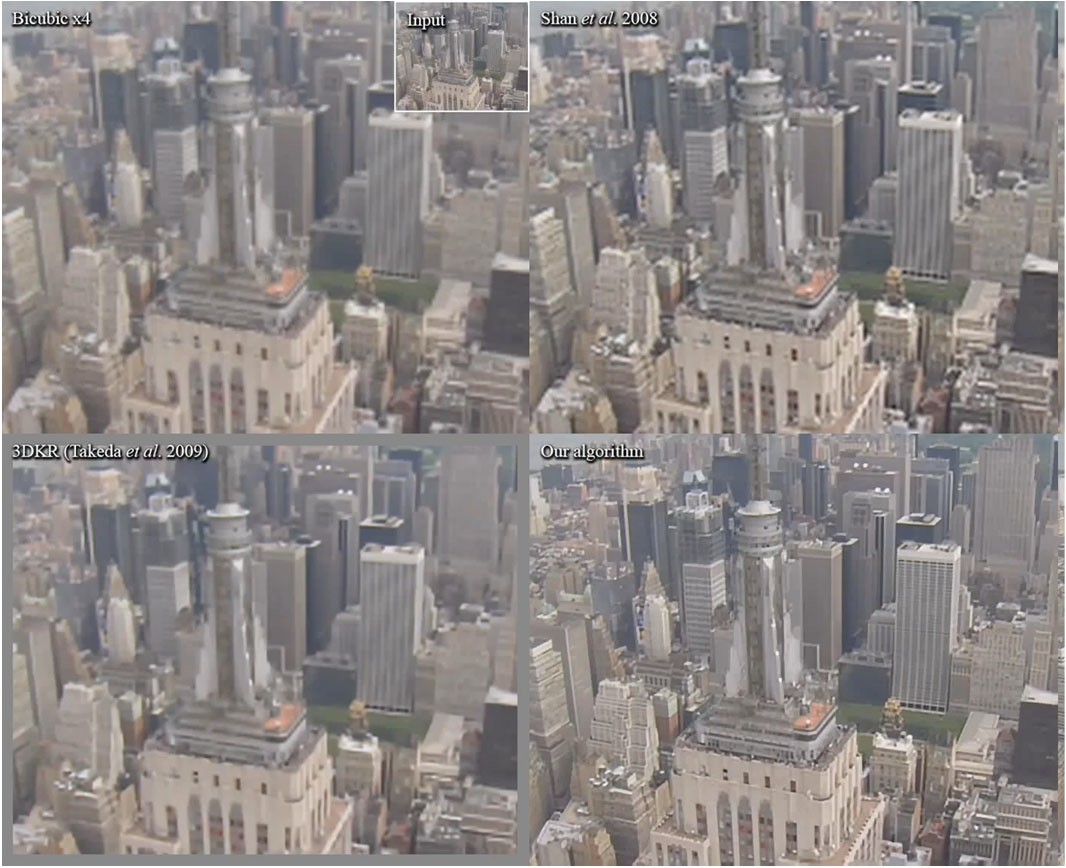
Liu & Sun, CVPR 2011; TPAMI 2014
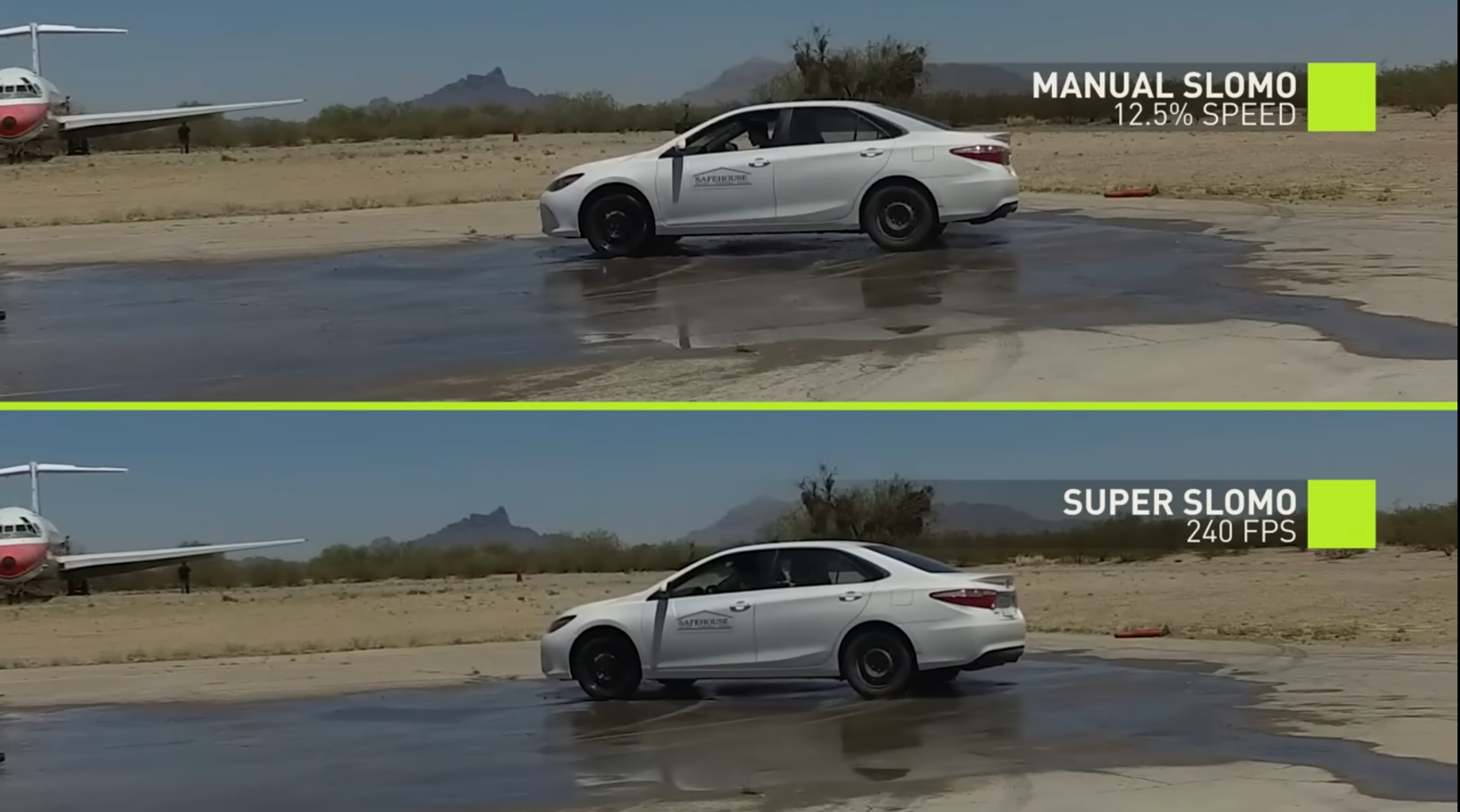
Super Slow Motion

Jiang et al., CVPR 2018
Watch on YouTube

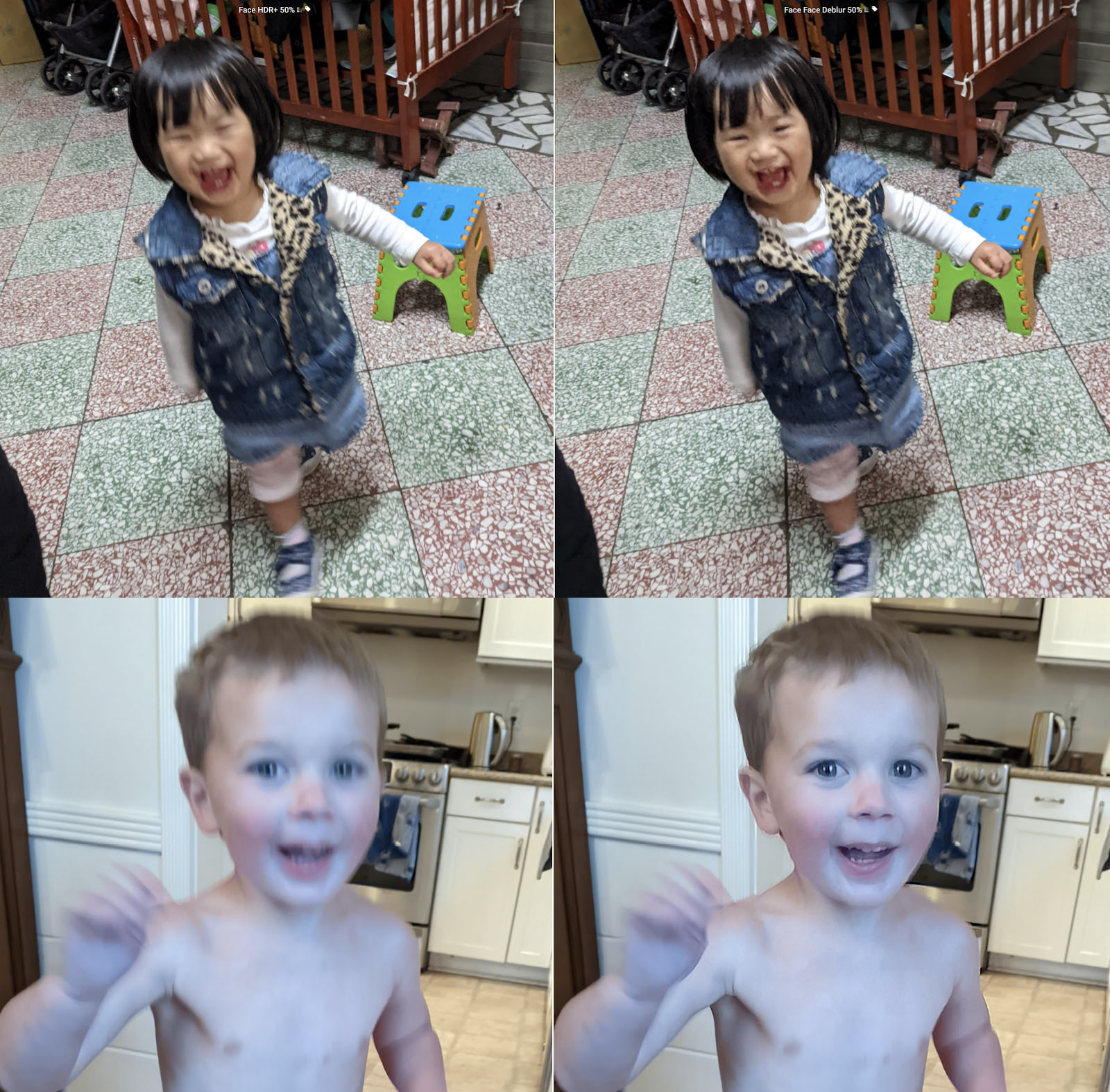
Image Unblur

Google Pixel 6: Face Unblur

Can We Use Feature Matching?

Can we estimate optical flow by detecting SIFT features and matching them between frames?

  • Yes—matched features provide sparse displacement estimates.
  • But an object may have no distinctive appearance separating it from its background.
Can you locate the hidden object? Click the texture or advance once.
Random texture with a hidden patch The moving texture region is outlined in red for print
Sometimes motion reveals structure that is difficult to see in a single frame.
Moving region outlined in red for print.

Can we estimate motion directly from changes in image intensity, without detecting and matching keypoints?

Brightness Constancy

What stays the same as a point moves between frames?

  • Brightness constancy: a scene point keeps its intensity as it moves: \[ I(x,y,t) = I(x+u,\ y+v,\ t+1) \]
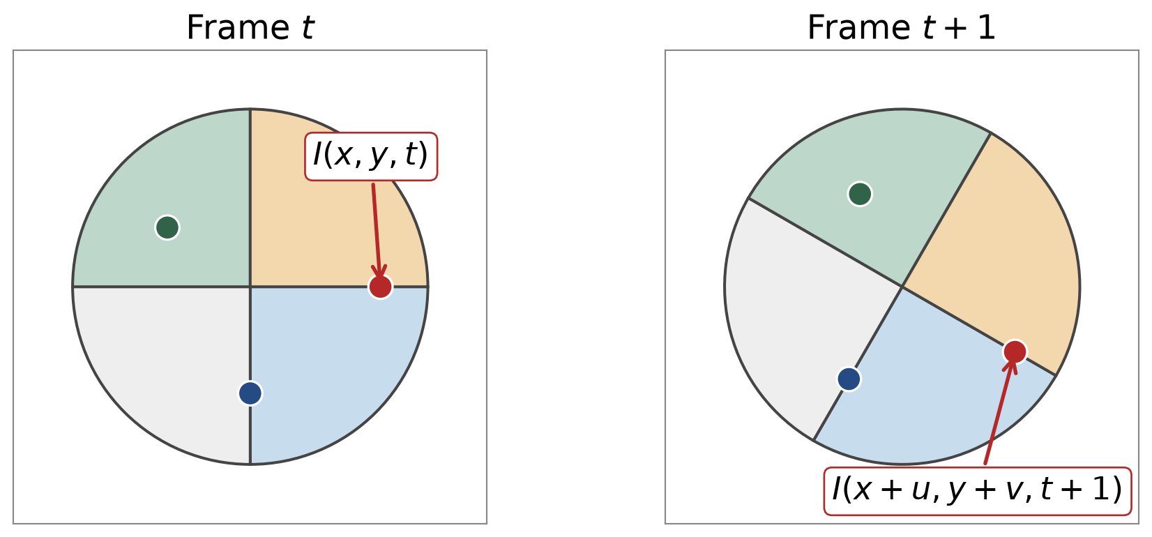
  • The marked point has the same intensity in both frames; only its position changes.
  • Brightness constancy holds when lighting is constant, the surface looks the same from slightly different viewpoints, and the frames are close in time.

Optical Flow Equation

Rearrange brightness constancy and apply a first-order Taylor expansion:

\[ \begin{aligned} 0 &= I(x+u,y+v,t+1) - I(x,y,t)\\[2pt] &\approx I(x,y,t) + I_x u + I_y v + I_t - I(x,y,t)\\[2pt] &= I_x u + I_y v + I_t\\[2pt] &= \nabla I \cdot [u,\ v]^T + I_t \end{aligned} \]

  • \(I_x, I_y\): spatial image gradients.
  • \(I_t \approx I(x,y,t+1) - I(x,y,t)\): change of intensity at a fixed pixel.

Optical Flow Equation

\[ I_x u + I_y v + I_t = 0 \]

When is this approximation bad? When \(u\) or \(v\) is large compared with how smoothly the image varies.

Why Do Spatial Gradients Reveal Motion?

What do static image gradients have to do with motion?

  • Consider a 1D intensity profile that shifts right by \(u\) pixels. Brightness constancy simplifies to \(I_x u + I_t = 0\).
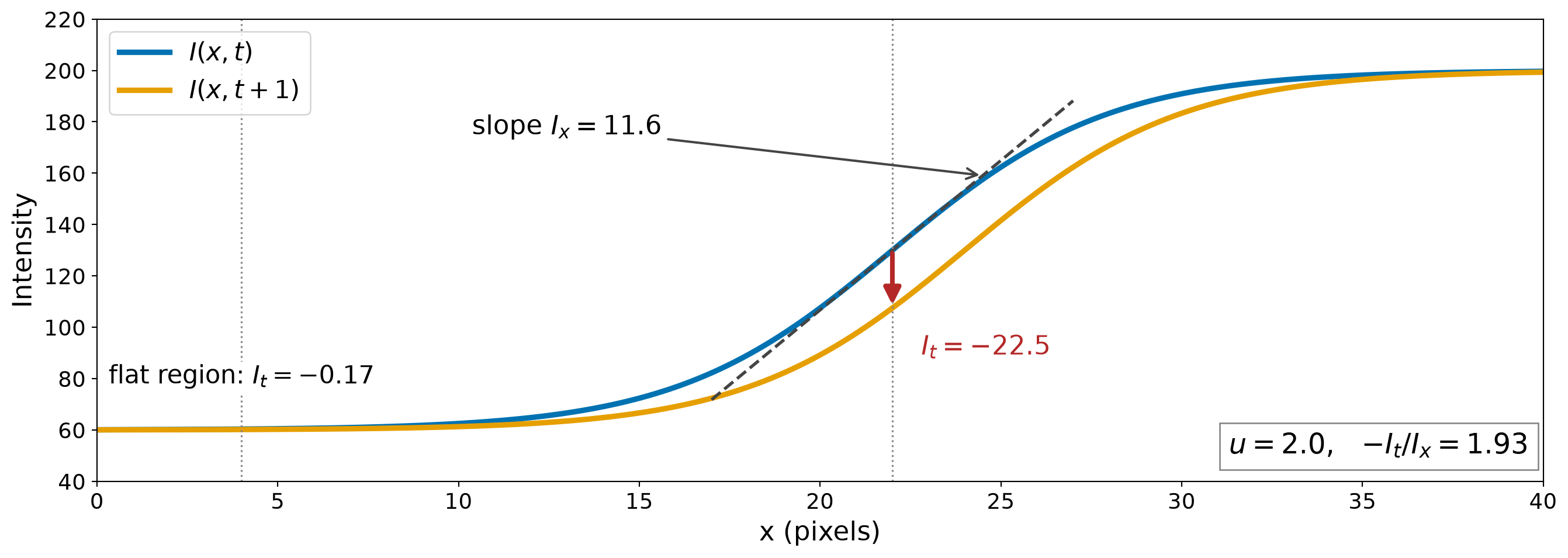
  • On a slope, shifting the profile changes the intensity at a fixed pixel by about \(-I_x u\), so \(u \approx -I_t/I_x\).
  • In a flat region, the intensity barely changes: the motion is nearly invisible.

Brightness Constancy Example
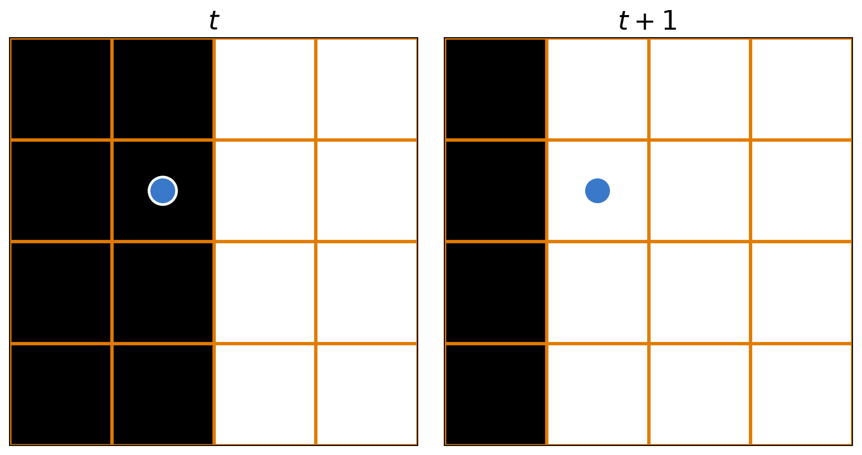
Pixel values: black = 0, white = 1. Derivatives use forward differences.

\[I_x = 1,\qquad I_y = 0,\qquad I_t = 1\]

\[I_x u + I_y v + I_t = 0\] \[\Rightarrow\; 1\,u + 0\,v + 1 = 0\]

  • What’s \(u\)?
    • \(u = -I_t/I_x = -1\): the edge moved one pixel left.
  • What’s \(v\)?
    • Any value satisfies the equation. Vertical motion of a vertical edge leaves no trace.

The Aperture Problem

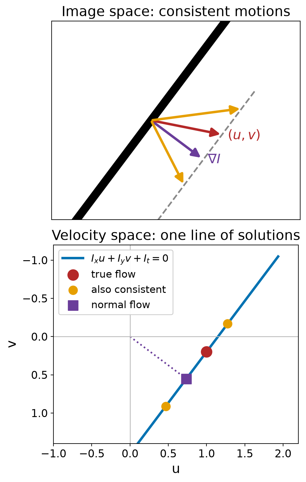
If Lucas–Kanade window sees only a straight edge, many different motions look the same:

Optical flow animation
  • Inside the aperture, only motion perpendicular to the edge is observable.

One Equation, Two Unknowns

Given \(I_x, I_y, I_t\), can we uniquely recover \((u,v)\) from the optical flow equation \(I_x u + I_y v + I_t = 0\)?

  • No: one equation per pixel, two unknowns.
  • If \((u,v)\) satisfies \(\nabla I\cdot(u,v) + I_t = 0\), so does \((u+u',\ v+v')\) for any \((u',v')\) with \(\nabla I\cdot(u',v') = 0\).
  • Only the flow component along the gradient can be recovered: \[ u_n = -\frac{I_t}{\lVert\nabla I\rVert} \]
  • The component parallel to the edge is lost.
Lucas–Kanade: More Equations from a Window

  • Each pixel gives 1 equation and 2 unknowns. How do we get more equations?
  • Assume spatial coherence: pixels in a small window move together and share the same \((u,v)\).
  • A \(5\times5\) window gives 25 equations:

\[ \underbrace{\begin{bmatrix} I_x(p_1) & I_y(p_1)\\ \vdots & \vdots\\ I_x(p_{25}) & I_y(p_{25}) \end{bmatrix}}_{A\ (25\times2)} \underbrace{\begin{bmatrix} u\\ v \end{bmatrix}}_{\mathbf d\ (2\times1)} = \underbrace{-\begin{bmatrix} I_t(p_1)\\ \vdots\\ I_t(p_{25}) \end{bmatrix}}_{\mathbf b\ (25\times1)} \]

B. Lucas and T. Kanade, “An iterative image registration technique with an application to stereo vision,” IJCAI, 1981.
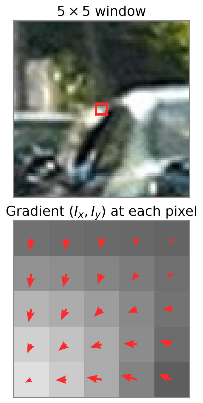
Frame 2 is a synthetic shift of image by \((u,v)=(0.6,-0.4)\) px.

Solving for \((u,v)\)

Least squares:

\[ A^TA\,\mathbf d = A^T\mathbf b \quad\Rightarrow\quad \mathbf d = (A^TA)^{-1}A^T\mathbf b \]

Summing over the pixels in the window:

\[ \underbrace{\begin{bmatrix} \sum I_xI_x & \sum I_xI_y\\ \sum I_xI_y & \sum I_yI_y \end{bmatrix}}_{A^TA} \begin{bmatrix} u\\ v \end{bmatrix} = \underbrace{-\begin{bmatrix} \sum I_xI_t\\ \sum I_yI_t \end{bmatrix}}_{A^T\mathbf b} \]

  • Similar to the Hough transform, each pixel contributes a line in parameter space.
  • Least squares finds the \((u,v)\) that best satisfies all lines.
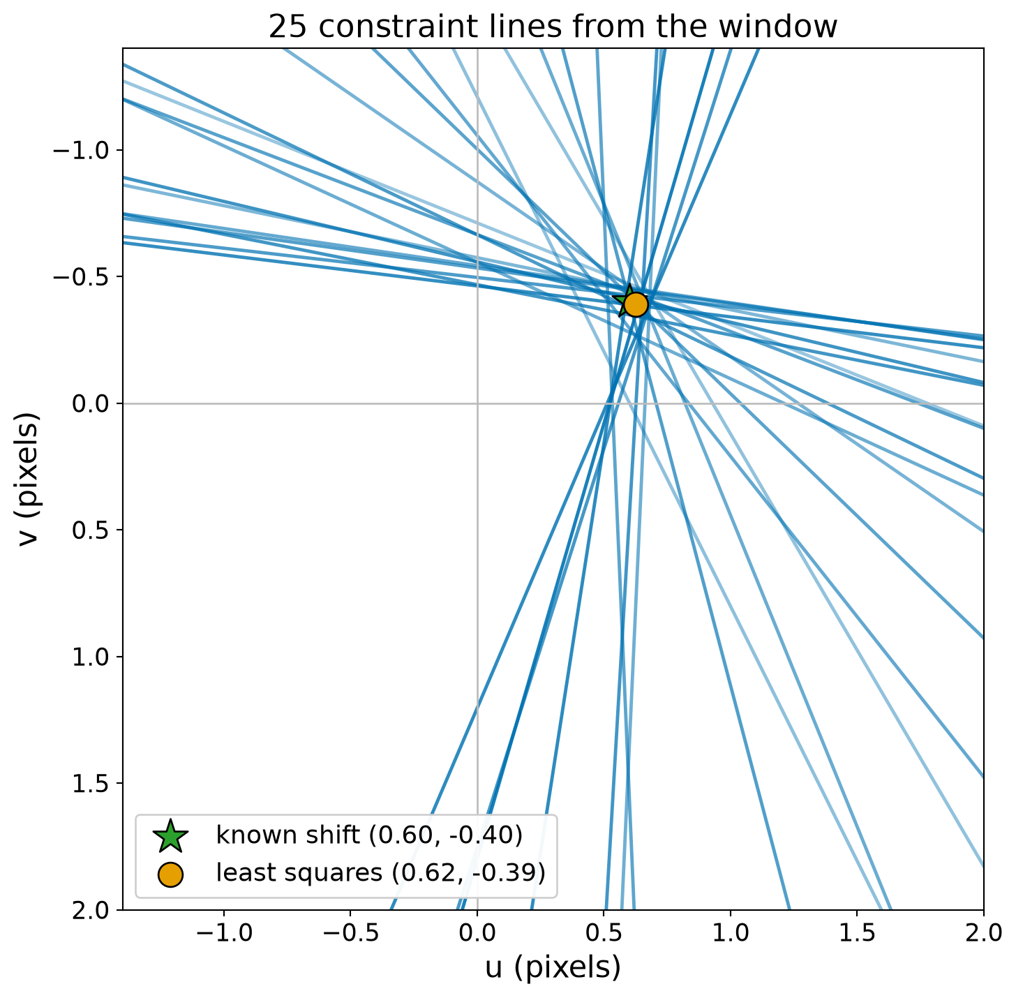
The \(v\) axis points down, as in image coordinates.

When Can We Solve for \((u,v)\)?

  • \(A^TA\) must be invertible: in a uniform region it is singular.
  • \(A^TA\) must not be too small: otherwise noise dominates.
  • \(A^TA\) must be well-conditioned: a large \(\lambda_1/\lambda_2\) indicates an edge.
  • \(A^TA\) is the second moment matrix \(M\) from Harris corners: good corners give reliable flow.
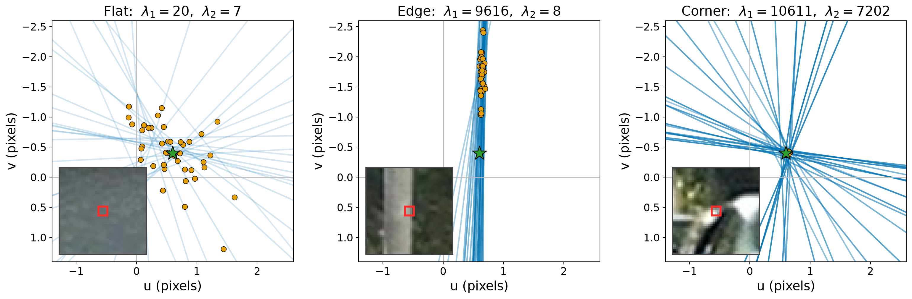
Orange dots: estimates from 40 frame pairs with independent noise. Green star: known shift. At the edge, \(u\) is accurate but \(v\) is not.

Lucas–Kanade Implementation

Lucas–Kanade (one window)

  1. Compute \(I_x, I_y\) from a smoothed frame and \(I_t\) from the frame difference.
  2. Sum products over the window to form \(A^TA\) and \(A^T\mathbf b\).
  3. Skip the window if the smaller eigenvalue of \(A^TA\) is too small.
  4. Solve the \(2\times2\) system for \((u,v)\).

Simplified implementation:

def lucas_kanade_window(frame1, frame2, x, y, half_size=2, min_eigenvalue=100):
    gradient_x, gradient_y = image_gradients(frame1)
    temporal_change = frame2 - frame1
    window = np.s_[y-half_size:y+half_size+1, x-half_size:x+half_size+1]
    Ix, Iy, It = gradient_x[window], gradient_y[window], temporal_change[window]

    ATA = np.array([[np.sum(Ix*Ix), np.sum(Ix*Iy)],
                    [np.sum(Ix*Iy), np.sum(Iy*Iy)]])
    ATb = -np.array([np.sum(Ix*It), np.sum(Iy*It)])

    if np.linalg.eigvalsh(ATA)[0] < min_eigenvalue:
        return None
    return np.linalg.solve(ATA, ATb)

When Does Lucas–Kanade Fail?

  • Large motion: the Taylor approximation breaks down.
  • Occlusions: points appear or disappear.
  • Lighting changes, noise: brightness constancy is violated.
  • Textureless regions: \(A^TA\) is nearly singular.
  • Edges (aperture problem): \(A^TA\) is ill-conditioned.
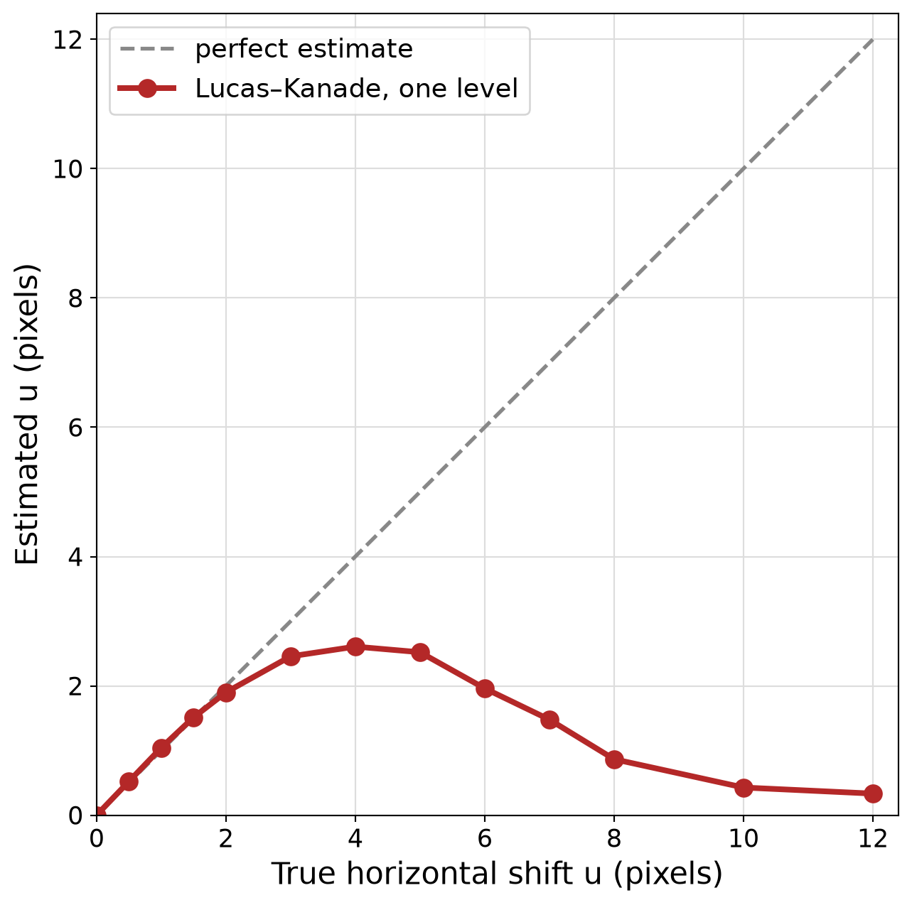
Synthetic horizontal shifts of the street image; median estimate over the most textured \(5\times5\) windows.

Coarse-to-Fine Estimation

  • Each Gaussian pyramid level halves the image size, so it also halves the displacement.
  • At a coarse enough level, the motion is small enough for the linearization to hold.
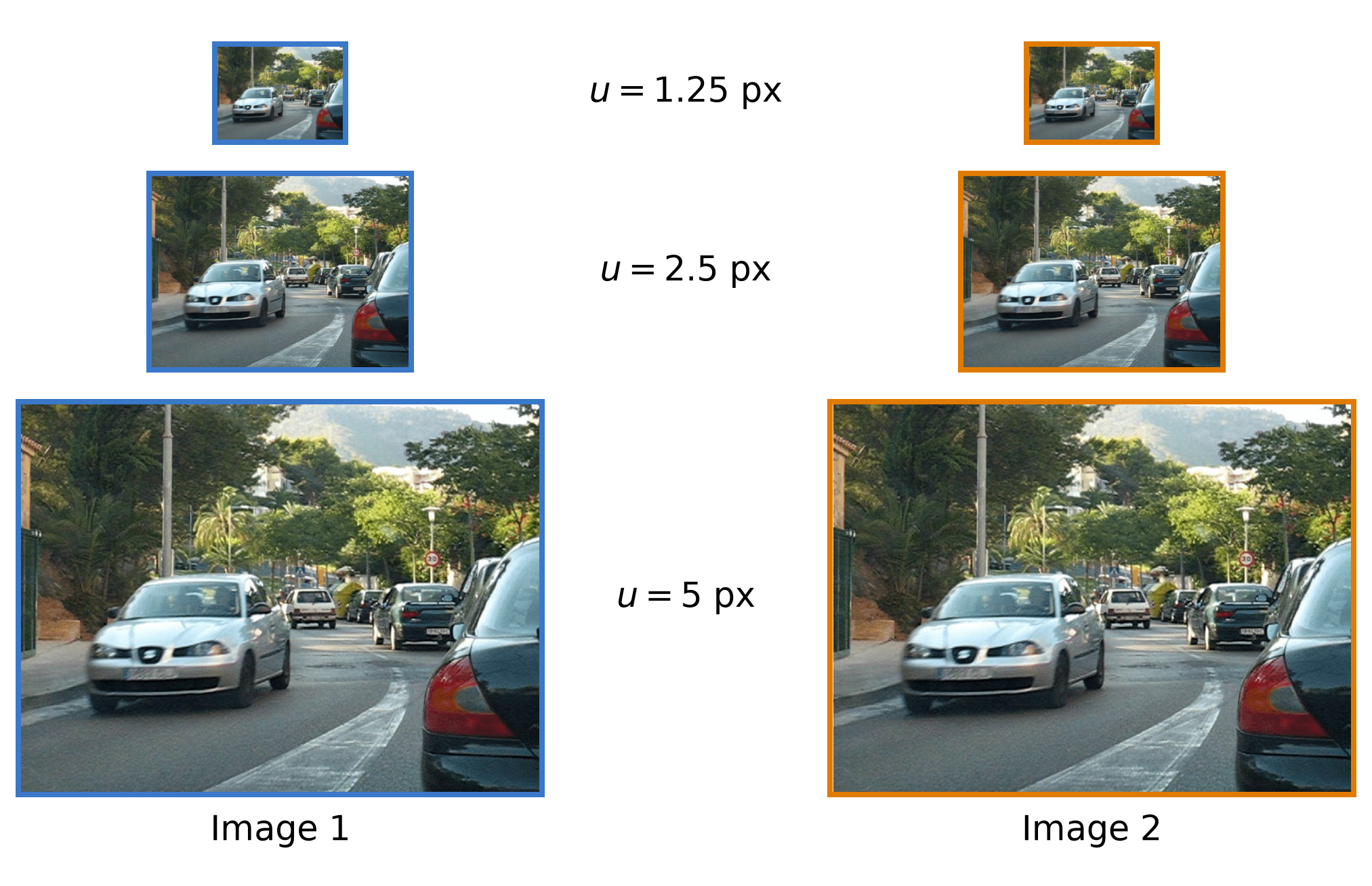
Coarse-to-Fine Algorithm

Coarse-to-Fine Lucas–Kanade

  1. Build Gaussian pyramids of both frames.
  2. Estimate flow at the coarsest level.
  3. Upsample the flow to the next level and double its values.
  4. Warp frame 2 toward frame 1 using the current flow.
  5. Estimate the remaining flow with Lucas–Kanade and add it.
  6. Repeat until the finest level.

Warping uses the current flow estimate \((u_0,v_0)\) to resample frame 2, pulling each pixel back by the motion already found: \[ I_2^{\text{warped}}(x,y) = I_2(x+u_0,\ y+v_0) \]
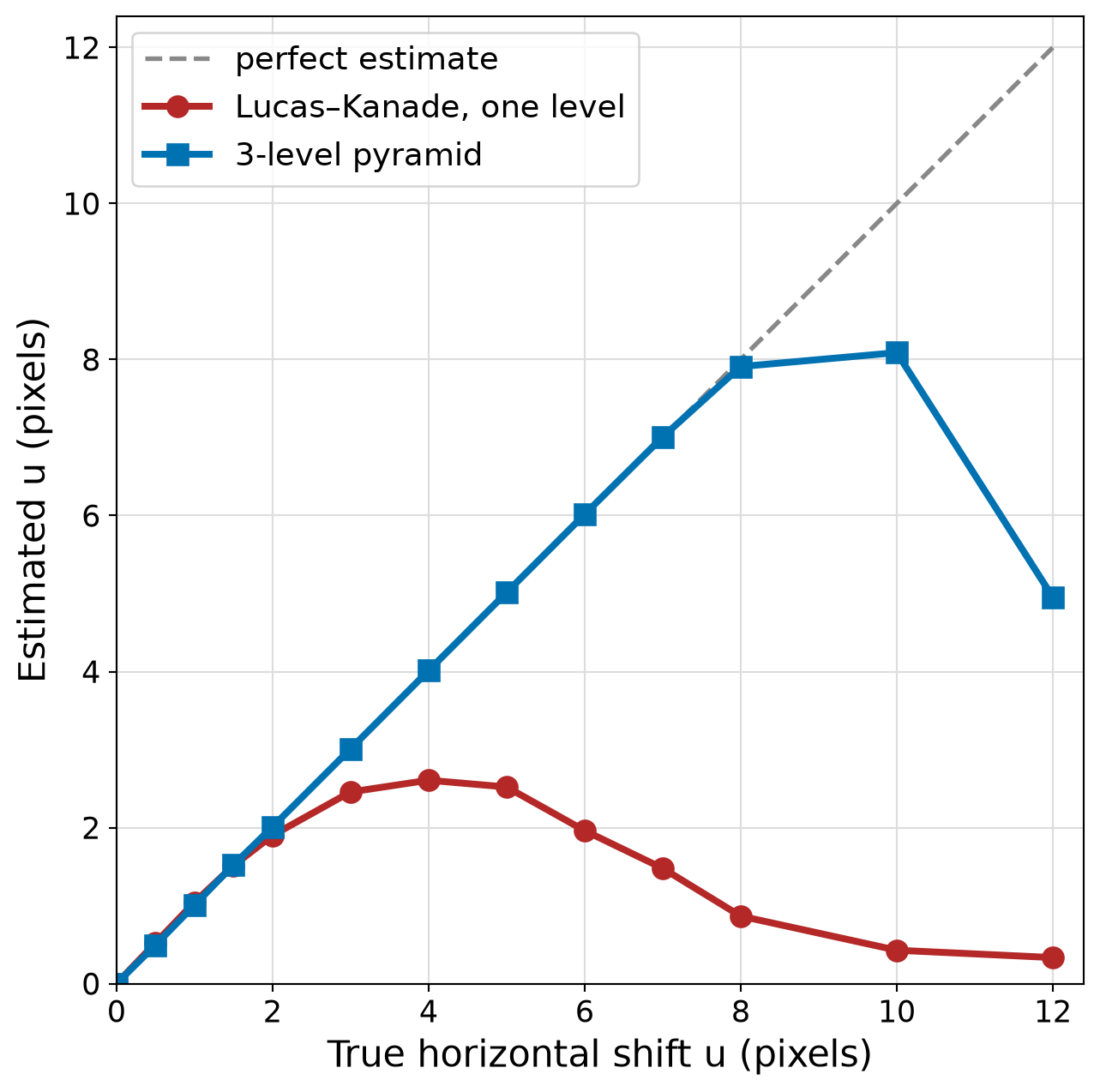
Same synthetic shifts as before. At the coarsest of 3 levels, an 8 px shift becomes 2 px.

Lucas–Kanade in OpenCV: Selecting Points

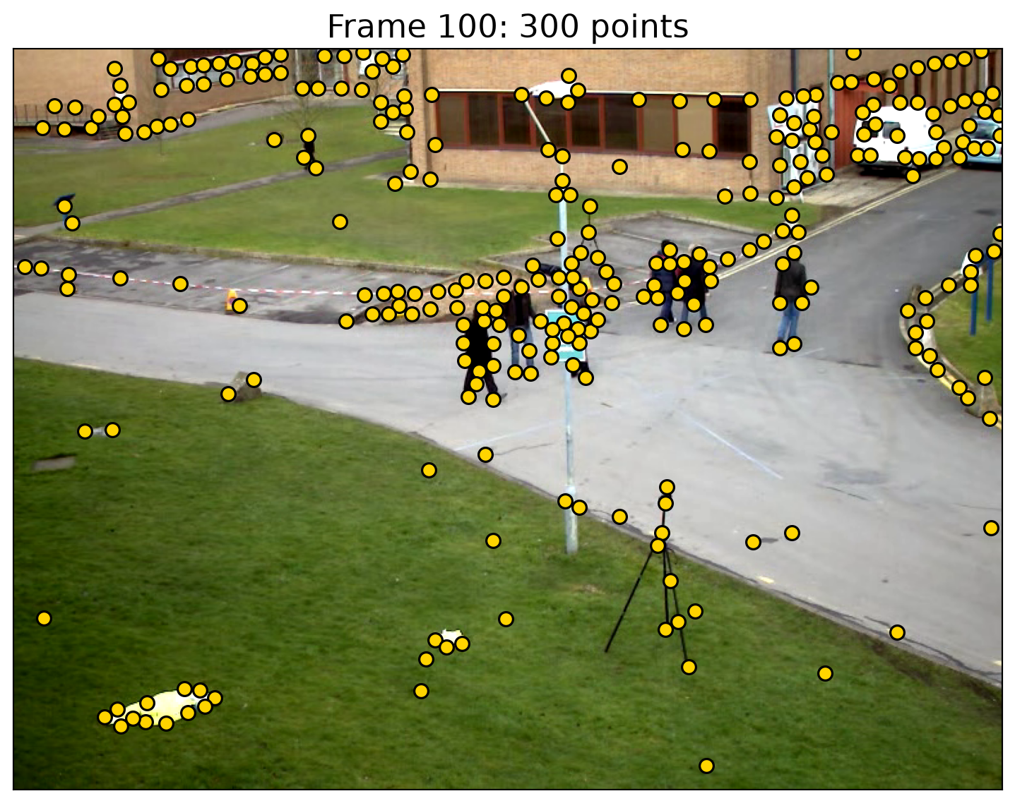
corners = cv2.goodFeaturesToTrack(
    gray1, maxCorners=300, qualityLevel=0.01,
    minDistance=10, blockSize=7)
  • Keeps points where the smaller eigenvalue of \(A^TA\) is large: the windows where Lucas–Kanade is solvable.
  • qualityLevel: keep points whose smaller eigenvalue is at least 1% of the strongest one.
  • minDistance: minimum spacing between points (pixels).
  • blockSize: window size used to form \(A^TA\).

Lucas–Kanade in OpenCV: Tracking

next_points, status, _ = cv2.calcOpticalFlowPyrLK(
    gray1, gray2, corners, None, winSize=(15, 15), maxLevel=3)

tracked = status.ravel() == 1
displacement = (next_points - corners)[tracked, 0]
  • winSize: the Lucas–Kanade window at each pyramid level.
  • maxLevel: number of pyramid levels above the original (0 = no pyramid).
  • status: 1 if the point was tracked; keep only those.
  • displacement: \((u,v)\) for each retained point.
  • OpenCV point arrays have shape \((N,1,2)\); [:, 0] gives an \((N,2)\) array of coordinates.
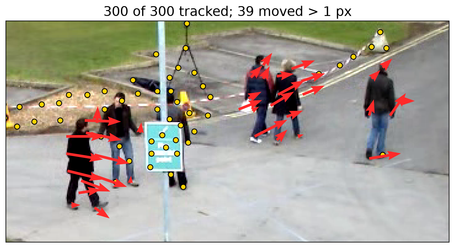
Frames 100 → 101, zoomed to the walkers. Arrows are drawn 5× longer than the displacement; yellow points moved ≤ 1 px.

Lucas–Kanade: Complete Video Example

import cv2
import numpy as np

GREEN, RED = (0, 255, 0), (0, 0, 255)  # OpenCV colors are BGR

def track_points(gray1, gray2, points):
    # Lucas-Kanade from gray1 to gray2, then back to gray1.
    next_points, status, error = cv2.calcOpticalFlowPyrLK(
        gray1, gray2, points, None, winSize=(15, 15), maxLevel=3)
    back_points, back_status, _ = cv2.calcOpticalFlowPyrLK(
        gray2, gray1, next_points, None, winSize=(15, 15), maxLevel=3)
    # Keep points found in both directions that came back within 1 px.
    returned = np.linalg.norm(points - back_points, axis=1) < 1
    tracked = (status.ravel() == 1) & (back_status.ravel() == 1) & returned
    return next_points, tracked

video = cv2.VideoCapture("vtest.avi")
tracks = []  # one track per point: its list of (x, y) positions
gray1 = None
frame_count = 0

while True:
    ok, frame = video.read()
    if not ok:  # end of the video
        break
    gray2 = cv2.cvtColor(frame, cv2.COLOR_BGR2GRAY)

    # Move each track's latest point to gray2; keep its last 10 positions.
    if gray1 is not None and tracks:
        points = np.float32([track[-1] for track in tracks])
        next_points, tracked = track_points(gray1, gray2, points)
        tracks = [(track + [point])[-10:] for track, point, keep
                  in zip(tracks, next_points, tracked) if keep]

    # Every 10 frames, add new points at least 10 px from those already tracked.
    if frame_count % 10 == 0:
        mask = np.full(gray2.shape, 255, np.uint8)
        for track in tracks:
            cv2.circle(mask, np.int32(track[-1]), 10, 0, -1)
        corners = cv2.goodFeaturesToTrack(gray2, maxCorners=300, qualityLevel=0.01,
                                          minDistance=10, blockSize=7, mask=mask)
        tracks += [[point] for point in corners[:, 0]]

    # Draw tails (green) and current positions (red).
    for track in tracks:
        cv2.polylines(frame, [np.int32(track)], False, GREEN, 2, cv2.LINE_AA)
        cv2.circle(frame, np.int32(track[-1]), 2, RED, -1, cv2.LINE_AA)
    cv2.imshow("Lucas-Kanade tracking", frame)
    if cv2.waitKey(100) == 27:  # 100 ms per frame (10 fps); Esc quits
        break

    gray1 = gray2
    frame_count += 1

video.release()
cv2.destroyAllWindows()

Tracking Points Through the Video

  • Track forward and backward; retain points that return within 1 px of their starting positions.
  • Green tails show each point’s last 10 positions; red dots show current positions.
  • Every 10 frames, detect new points away from those already tracked.
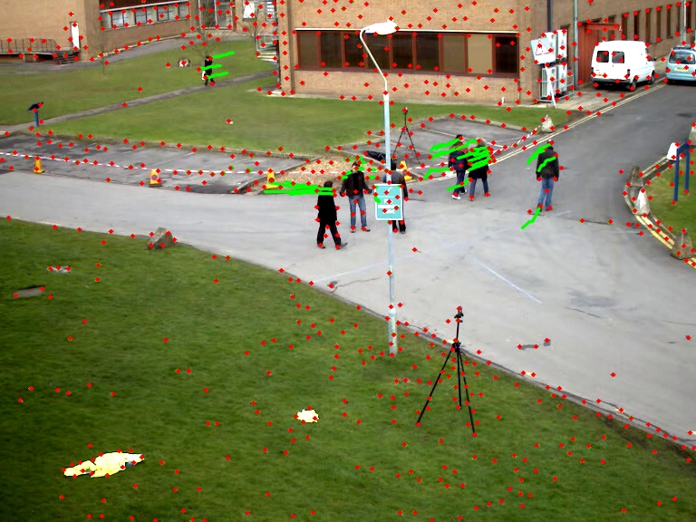
Lucas–Kanade trajectories with forward–backward filtering

Dense Optical Flow: Farnebäck

flow = cv2.calcOpticalFlowFarneback(
    gray1, gray2, None, pyr_scale=0.5, levels=3, winsize=15,
    iterations=3, poly_n=5, poly_sigma=1.2, flags=0)
  • flow has shape (height, width, 2): flow[y, x] \(=(u,v)\) at every pixel.
  • Fits a quadratic polynomial to each neighborhood and estimates how it shifts between frames.
  • pyr_scale: scale factor between pyramid levels.
  • levels: total number of levels, including the original image.
  • winsize: averaging window; larger is smoother and more robust to noise, but blurs motion boundaries.
  • iterations: refinements per pyramid level.
  • poly_n, poly_sigma: neighborhood size and smoothing for the polynomial fit.
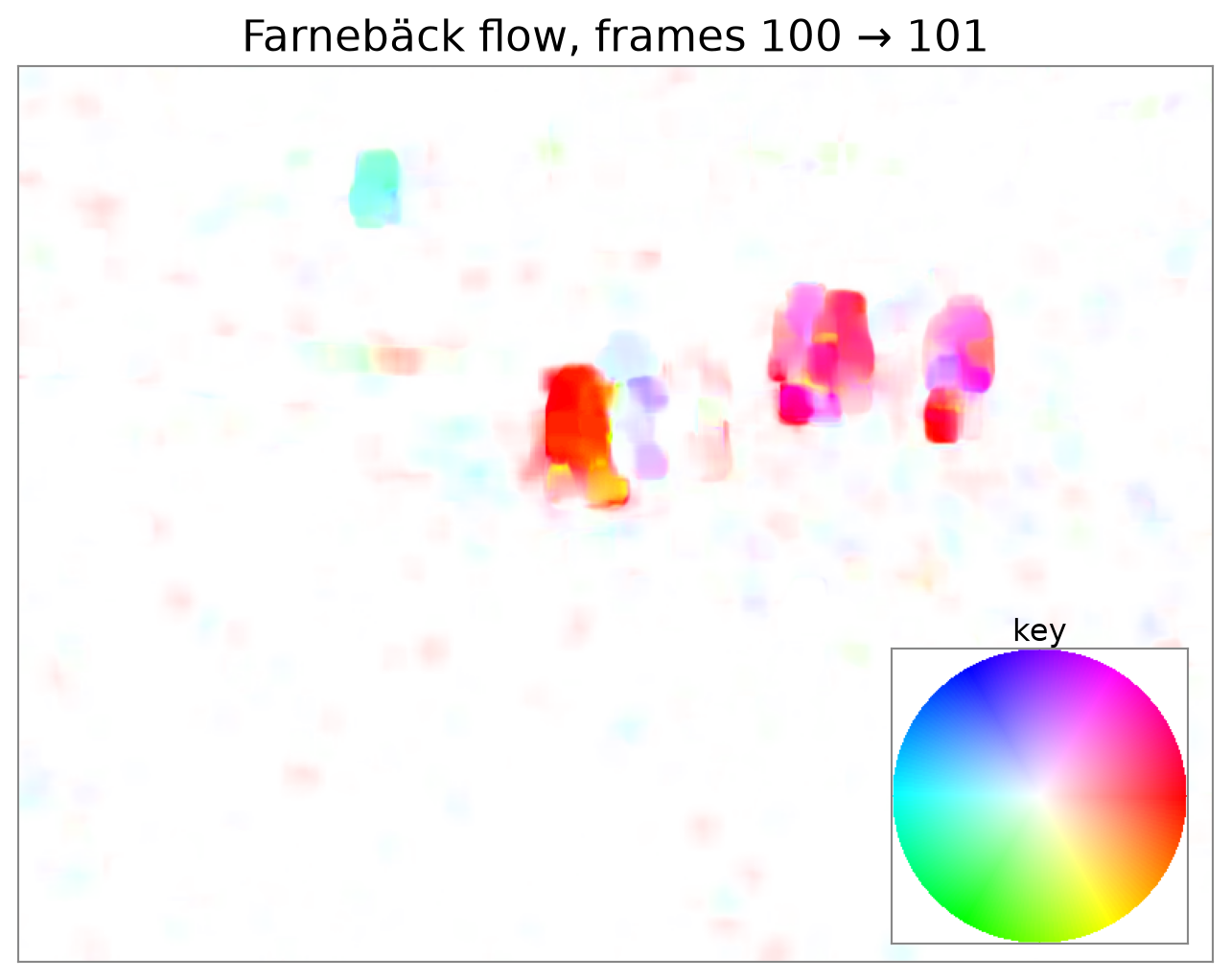
Hue: direction; saturation: magnitude, saturating at 5 px. White means no motion.

Dense Optical Flow: DIS

dis = cv2.DISOpticalFlow_create(cv2.DISOPTICAL_FLOW_PRESET_MEDIUM)
flow = dis.calc(gray1, gray2, None)
  • DIS: Dense Inverse Search.
  • Runs a fast Lucas–Kanade-style search on a grid of patches, then combines and refines their motion estimates into a dense field.
  • Presets (ULTRAFAST, FAST, MEDIUM) trade accuracy for speed.
  • Returns the same (height, width, 2) flow array format as Farnebäck.
  • Use the same color scale to compare the two methods.
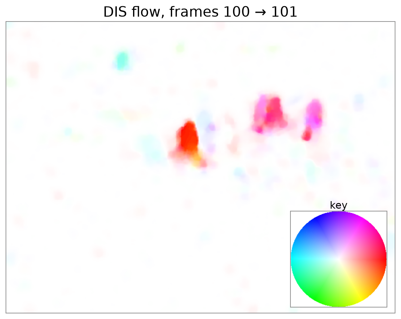
Hue: direction; saturation: magnitude, saturating at 5 px. White means no motion.

Dense Optical Flow: Complete Video Example

import cv2
import numpy as np

def flow_to_bgr(flow, max_flow=5):
    # Hue: direction. Saturation: magnitude. White: no motion.
    magnitude, angle = cv2.cartToPolar(
        flow[..., 0], flow[..., 1], angleInDegrees=True)
    hsv = np.zeros(flow.shape[:2] + (3,), np.uint8)
    hsv[..., 0] = angle / 2
    hsv[..., 1] = np.clip(255 * magnitude / max_flow, 0, 255)
    hsv[..., 2] = 255
    return cv2.cvtColor(hsv, cv2.COLOR_HSV2BGR)

video = cv2.VideoCapture("vtest.avi")
dis = cv2.DISOpticalFlow_create(cv2.DISOPTICAL_FLOW_PRESET_MEDIUM)

_, previous = video.read()
gray1 = cv2.cvtColor(previous, cv2.COLOR_BGR2GRAY)

while True:
    ok, current = video.read()
    if not ok:
        break
    gray2 = cv2.cvtColor(current, cv2.COLOR_BGR2GRAY)

    farneback = cv2.calcOpticalFlowFarneback(
        gray1, gray2, None, pyr_scale=0.5, levels=3, winsize=15,
        iterations=3, poly_n=5, poly_sigma=1.2, flags=0)
    dis_flow = dis.calc(gray1, gray2, None)

    # Forward flow is defined at pixels in the previous frame.
    cv2.imshow("Video", previous)
    cv2.imshow("Farneback", flow_to_bgr(farneback))
    cv2.imshow("DIS", flow_to_bgr(dis_flow))

    previous, gray1 = current, gray2
    if cv2.waitKey(100) == 27:  # Esc quits.
        break

video.release()
cv2.destroyAllWindows()

Comparing Dense Optical Flow

  • Both methods estimate motion at every pixel between consecutive frames.
  • Compare the walkers, motion boundaries, and nearly stationary background.
  • Both displays use the same color scale: white means no motion; saturation reaches its maximum at 5 px.
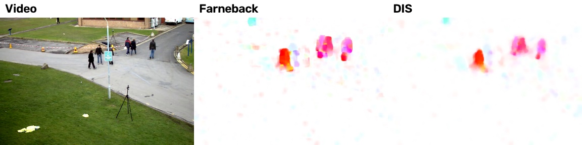
Video, Farnebäck flow, and DIS flow

Optical Flow in OpenCV

Method Function Output Module
Pyramidal Lucas–Kanade cv2.calcOpticalFlowPyrLK Sparse main
Farnebäck cv2.calcOpticalFlowFarneback Dense main
DIS cv2.DISOpticalFlow_create Dense main
Dual TV-L1 cv2.optflow.DualTVL1OpticalFlow_create Dense contrib
DeepFlow cv2.optflow.createOptFlow_DeepFlow Dense contrib
Sparse-to-dense cv2.optflow.calcOpticalFlowSparseToDense Dense contrib
Robust local flow (RLOF) cv2.optflow.calcOpticalFlowSparseRLOF, cv2.optflow.calcOpticalFlowDenseRLOF Both contrib
  • Sparse: track selected points (e.g., for visual odometry).
  • Dense: a vector at every pixel (e.g., motion segmentation).
  • contrib methods require OpenCV built with the contrib modules.

Key Takeaways

  • Optical flow describes apparent motion between images. Sparse methods estimate motion at selected points; dense methods estimate a vector at every pixel.
  • Brightness constancy and a small-motion approximation give \(I_xu + I_yv + I_t = 0\): one equation for two unknowns.
  • Lucas–Kanade assumes shared motion within a small window and combines its pixel equations using least squares. Reliable estimates require intensity variation in two directions—the same condition used to identify corners.
  • Coarse-to-fine estimation reduces apparent displacement, then refines the estimate through warping and residual motion updates.

When Is Motion Reliable?

Flat regions provide little motion information; a straight edge reveals only motion normal to the edge. Corners and texture help resolve both components, but lighting changes, occlusion, and large motion can still cause errors.