Lecture 11 — Camera Geometry
Lecture 11
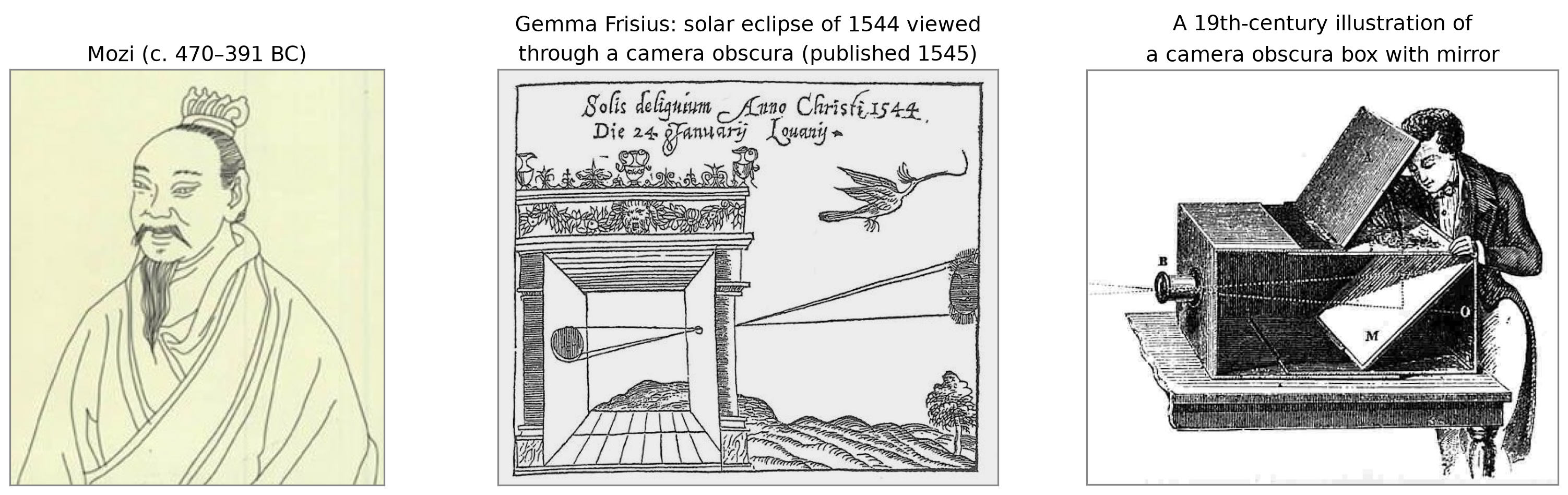
A Brief History: Recording the Image
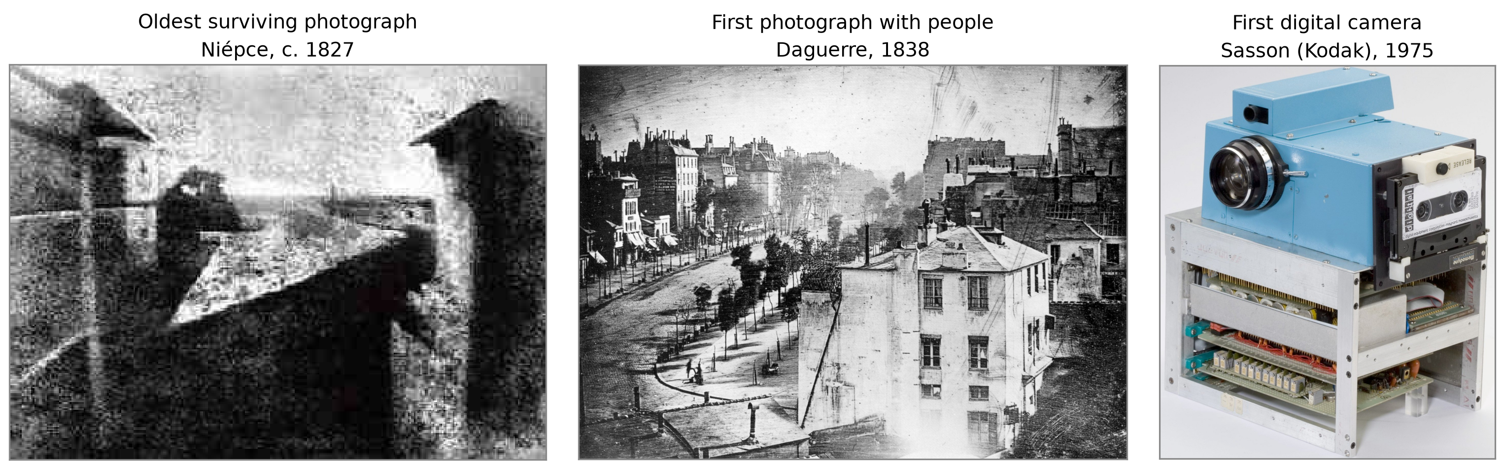
- Niépce: exposure of about 8 hours; held at the Harry Ransom Center, UT Austin.
- Daguerre: moving traffic left no trace; a man having his boots polished stood still long enough to appear.
- Sasson: \(100\times100\) pixels (0.01 megapixels), black and white, stored on cassette tape; 23 seconds per image, about 8 pounds.
Bare Sensor vs. Pinhole

- Bare sensor: every scene point reaches every pixel, so every pixel records nearly the same average color.
- Pinhole: the barrier blocks all but one ray from each point, so each pixel sees one scene point: an inverted image.
Pinhole Camera Terms
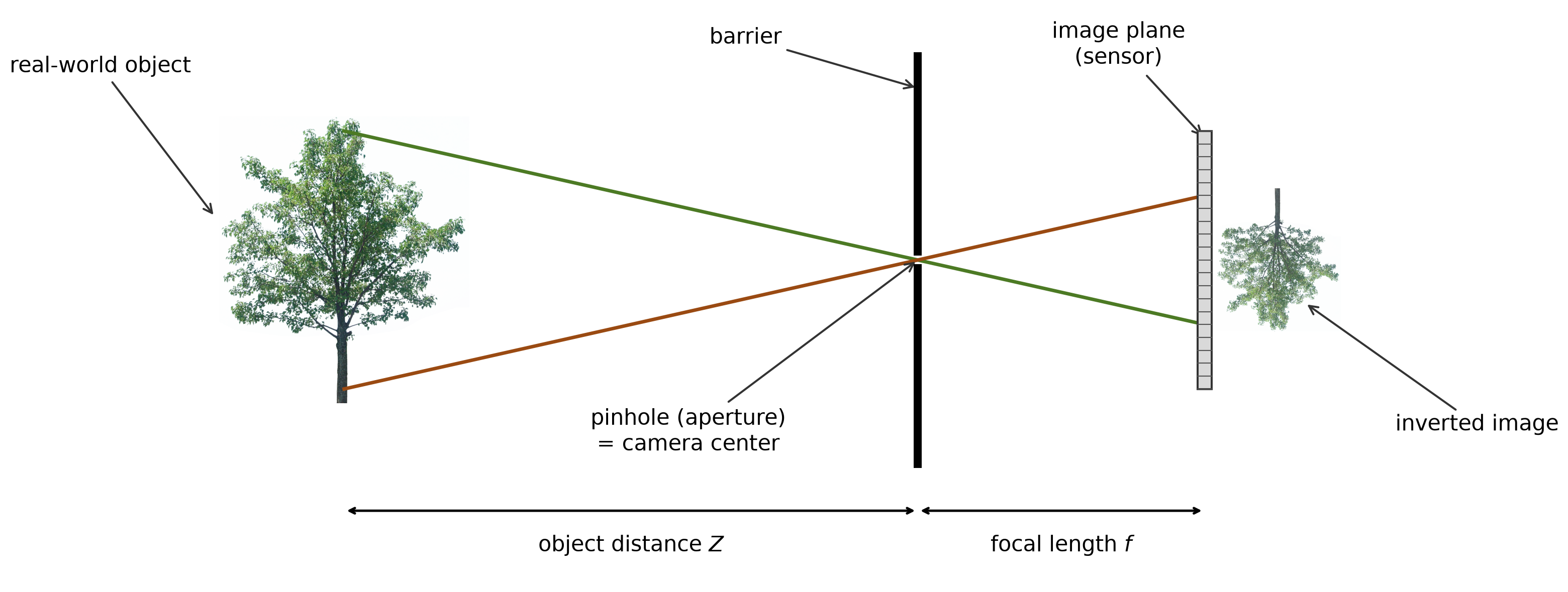
- The pinhole is the camera center (center of projection): every ray that forms the image passes through it.
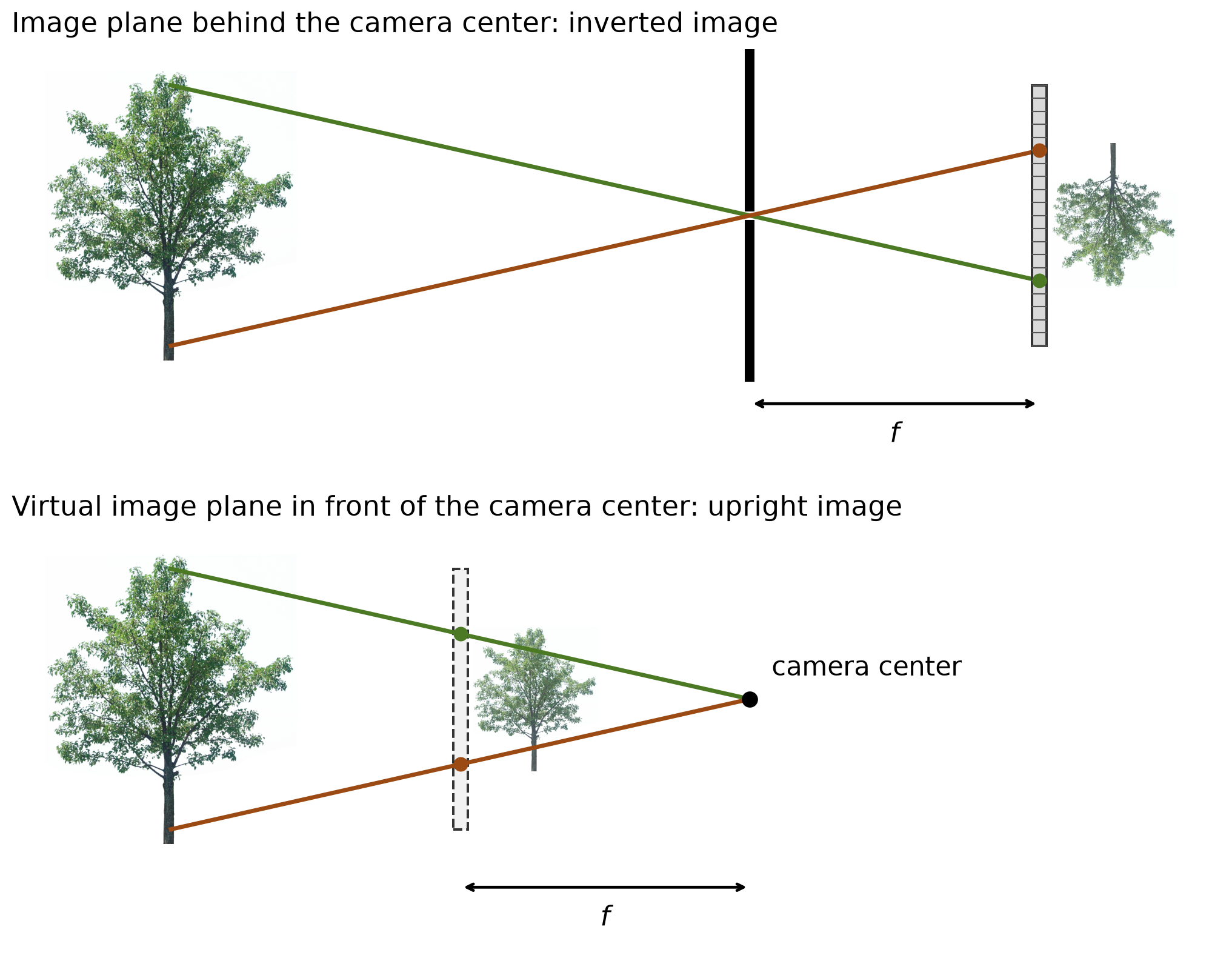
- The sensor lies in the image plane, a distance \(f\) (the focal length) behind the pinhole.
Focal Length

- Image size is \(f\,H/Z\): doubling \(f\) doubles the image and narrows the field of view.
- With the same pinhole, the light reaching each pixel is proportional to \(1/f^2\): doubling \(f\) gives ¼ of the light.
Pinhole Size: Sharpness vs. Light

- Light collected grows with the pinhole’s area (\(\propto d^2\)), but each scene point spreads over a spot of size \(\propto d\).
- A very small pinhole is sharp but dark; below a certain size, diffraction blurs the image again, so the pinhole cannot be made arbitrarily small.
The Lens Camera
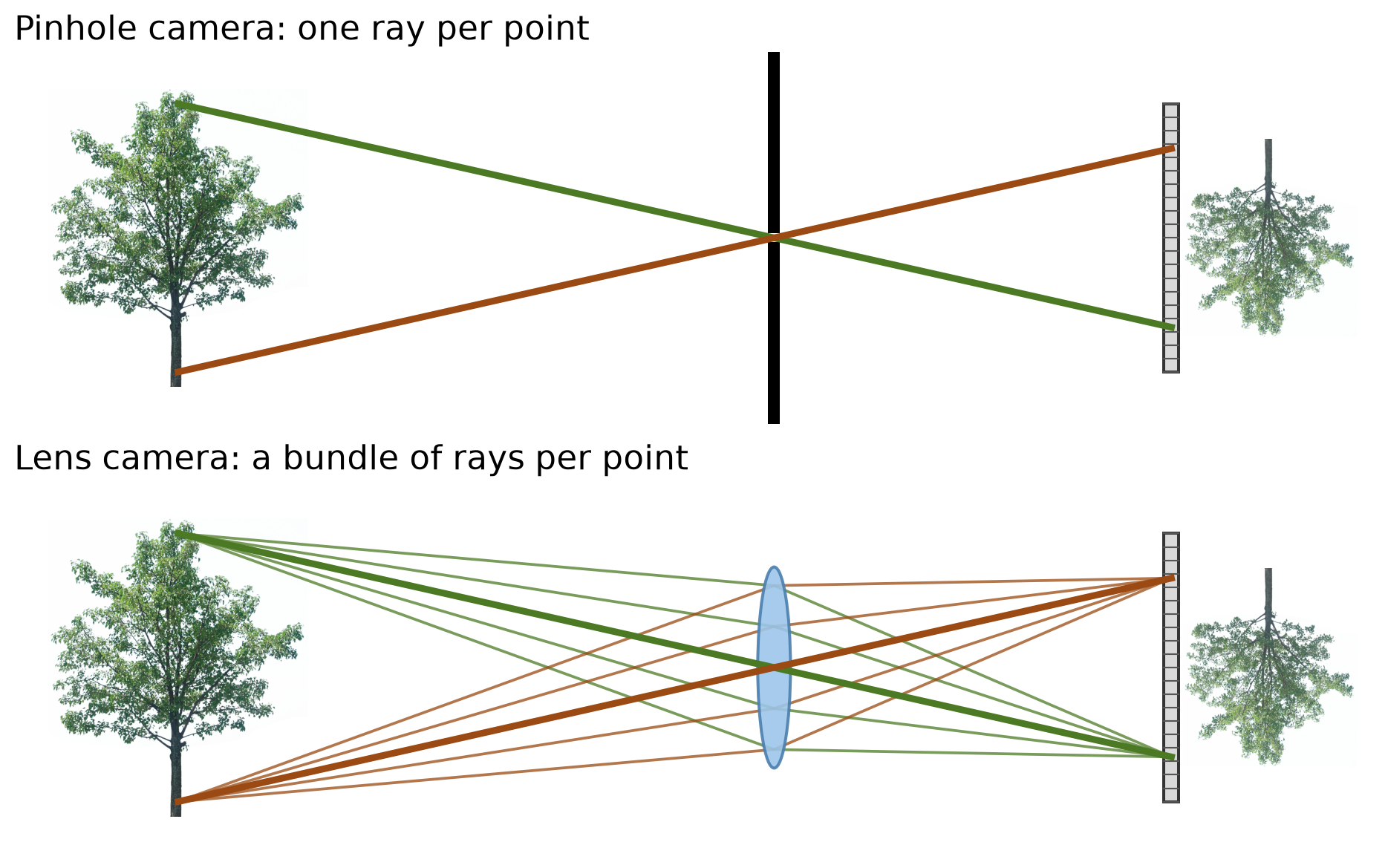
- A lens collects a bundle of rays from each scene point and focuses them back to one image point: far more light than a pinhole, without the blur.
- The central ray (thick) passes through the lens center undeflected, just as through a pinhole. When the lens is in focus, the pinhole model gives where each point lands.
Focal Length of a Lens
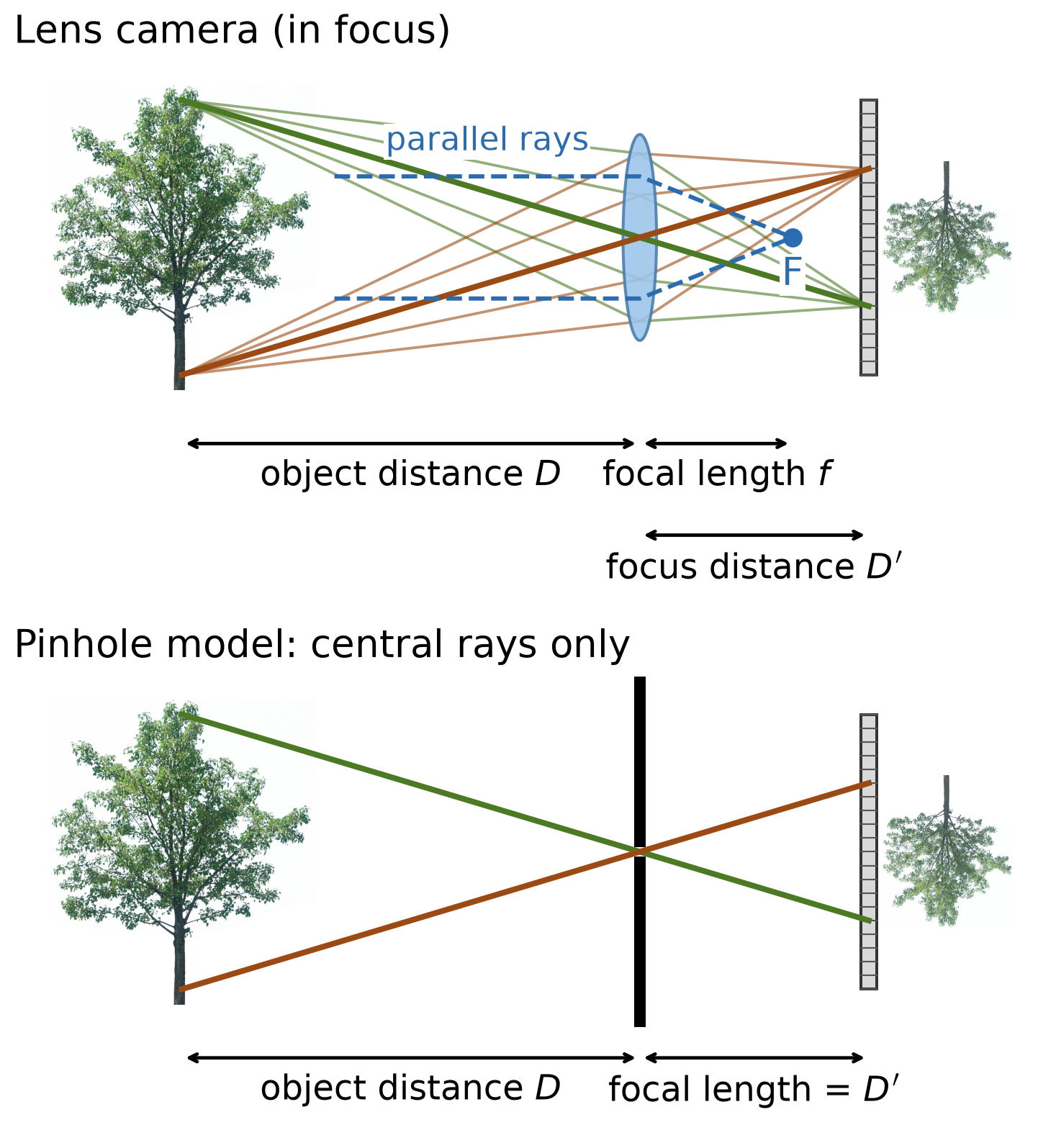
- In a lens camera, the focal length \(f\) is the distance at which parallel rays intersect (the focal point F).
- The image of an object at distance \(D\) forms at the focus distance \(D'\): \(\;\frac{1}{D} + \frac{1}{D'} = \frac{1}{f}\).
- The pinhole model describes a lens camera if:
- We use only central rays
- The lens is in focus
- The pinhole’s focal length equals the lens’s focus distance \(D'\); for a distant object, \(D' = f\).
- In this course, focal length \(f\) means the aperture–sensor distance, as in the pinhole camera.
The Virtual Image Plane
Placing a virtual image plane a distance \(f\) in front of the camera center gives the same image, the same size, but upright.
The virtual plane is mathematically equivalent and easier to work with, so from now on we will use it instead.
The Camera Coordinate Frame
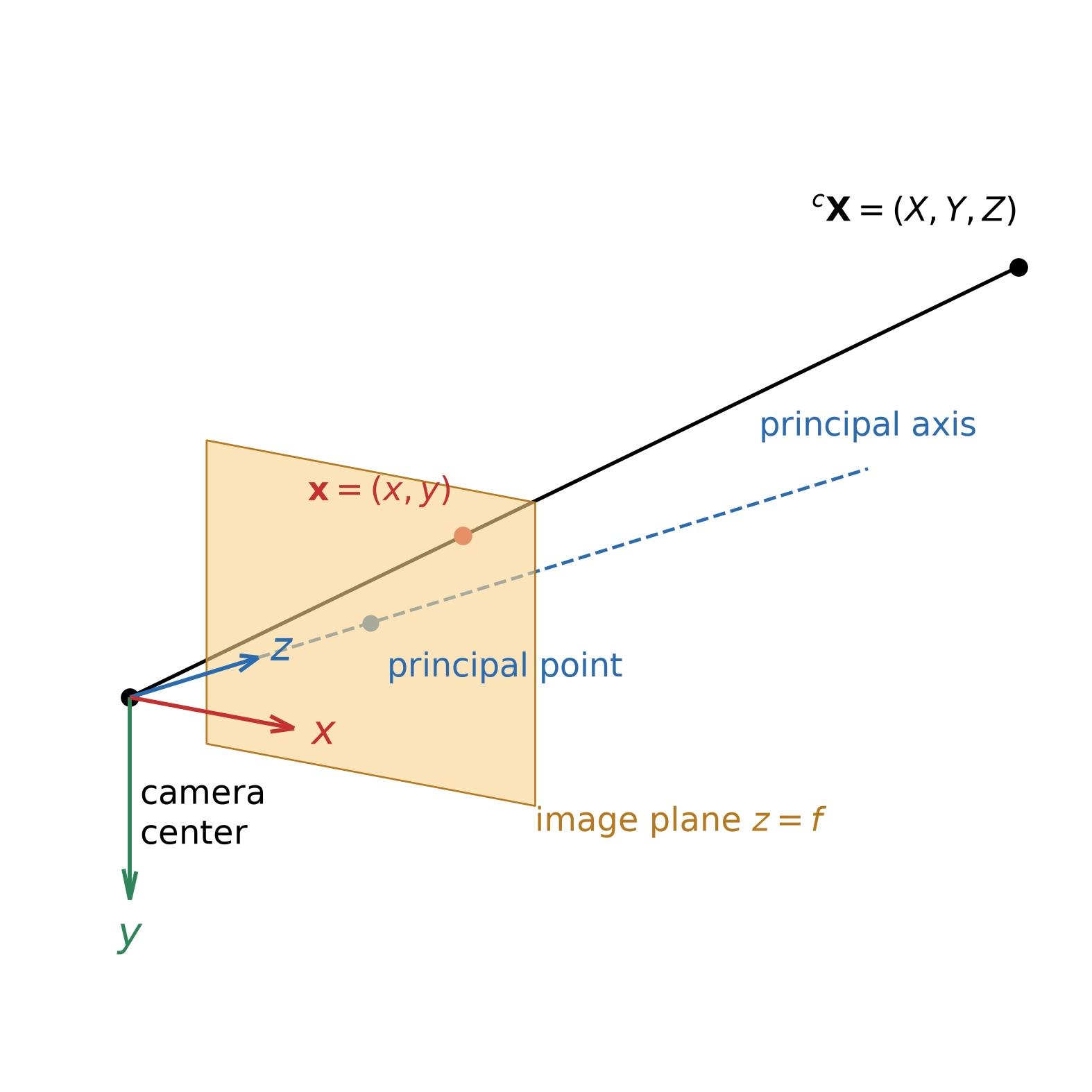
- Origin is at the camera center.
- Convention: \(x\) right, \(y\) down, \(z\) forward.
- The \(z\)-axis is the principal (optical) axis.
- The image plane is \(z = f\).
- The principal axis meets the image plane at the principal point.
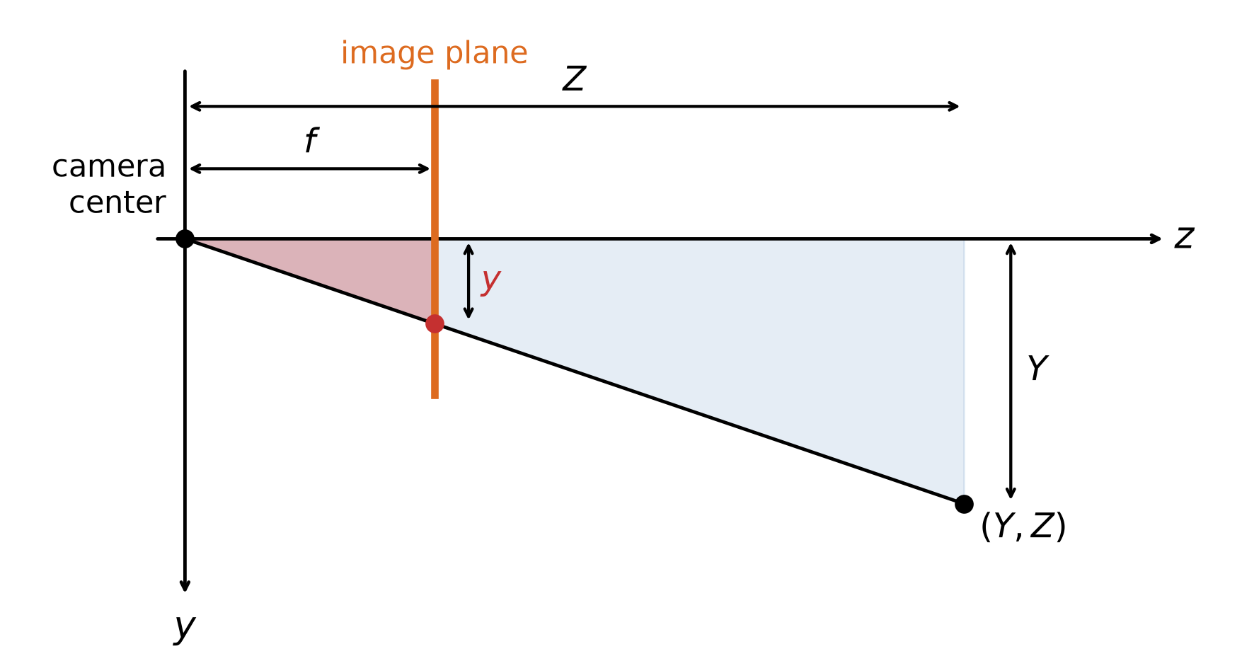
- A 3D point \({}^{c}\mathbf{X} = (X, Y, Z)\) in camera coordinates projects to the point \(\mathbf{x} = (x, y)\) where the ray to the camera center crosses the image plane.
Perspective Projection
Side view (\(y\)–\(z\) plane): the two shaded triangles are similar, so \[\frac{y}{f} = \frac{Y}{Z}, \qquad \text{and likewise} \qquad \frac{x}{f} = \frac{X}{Z}.\]
Perspective projection: \[(X,\ Y,\ Z) \;\mapsto\; \left(f\,\frac{X}{Z},\; f\,\frac{Y}{Z}\right)\]
The division by \(Z\) makes the projection nonlinear in \((X, Y, Z)\).
Homogeneous coordinates (defined later) will make it a matrix product.
Consequences of Perspective Projection

- Size \(\propto 1/Z\): doubling the distance halves the image of the cube.
- Depth is lost: every point on a ray through the camera center projects to the same image point.
- Vanishing points: parallel 3D lines (the rails) meet at one image point, on the horizon.
Consequences of Perspective Projection
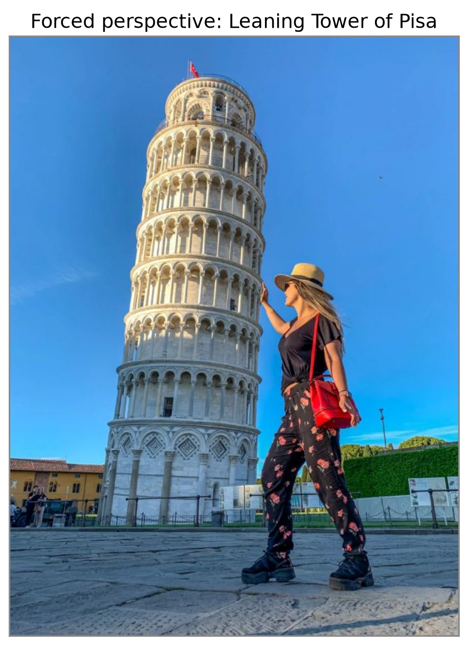
StruckDuck, Impossible Gravity Slide Illusion
Homogeneous Coordinates
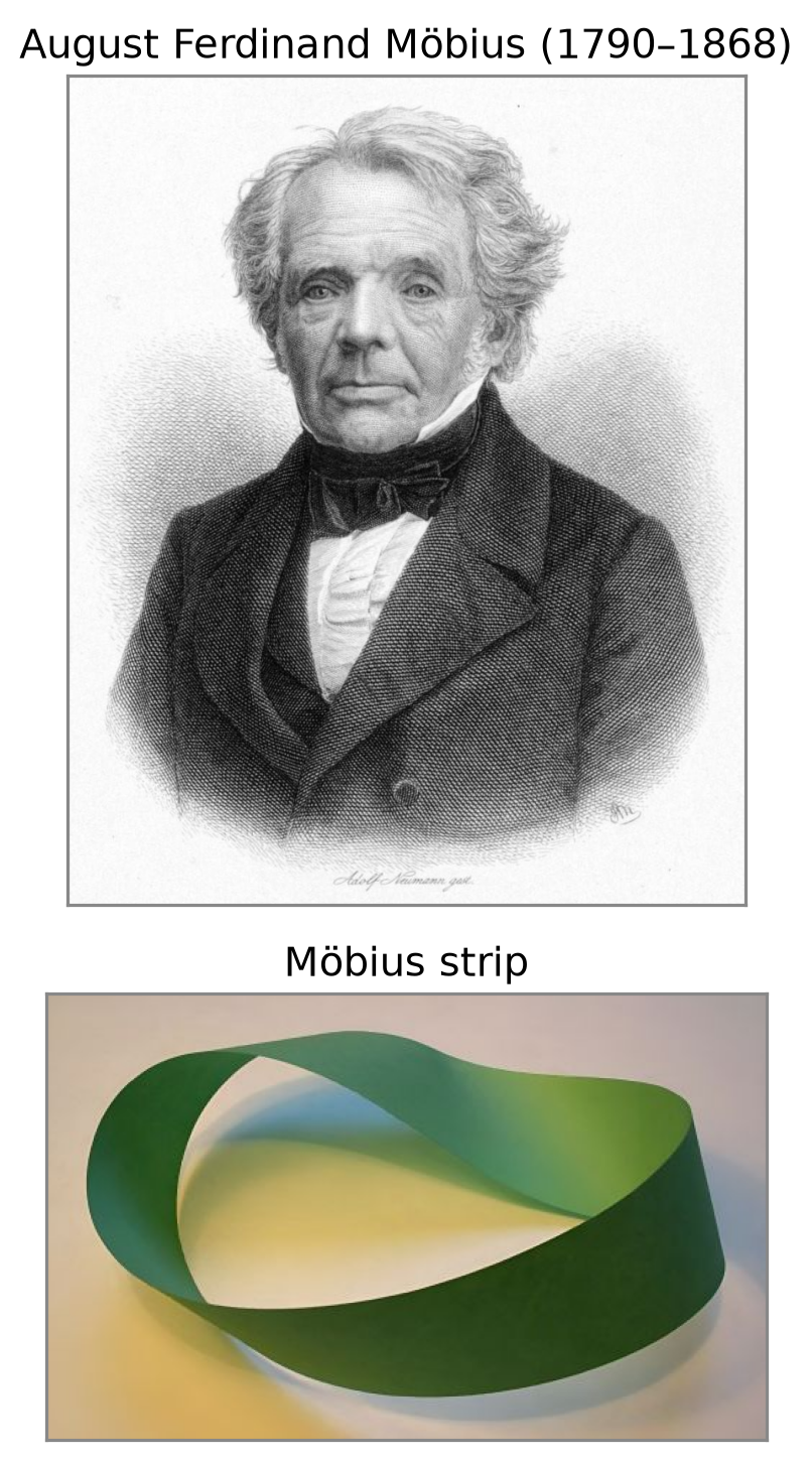
- Introduced by August Ferdinand Möbius (1827), as an alternative to Cartesian coordinates for projective geometry.
- Add one extra coordinate: a 2D point gets 3 numbers, a 3D point gets 4.
- Why we use them in computer vision:
- Translation becomes a matrix product
- Perspective projection becomes a matrix product
- A chain of transformations becomes a single matrix
A Point Is a Ray
- All multiples of a homogeneous vector are the same point: \[k\begin{bmatrix} x \\ y \\ w \end{bmatrix} \sim \begin{bmatrix} x \\ y \\ w \end{bmatrix}, \quad k \neq 0\]
- So a 2D point is a ray through the origin; its Cartesian coordinates are where the ray crosses the plane \(w = 1\).
- This is the pinhole camera: every 3D point on a ray through the camera center lands on the same image point (scale ambiguity).

Parametric (Global) Transformations
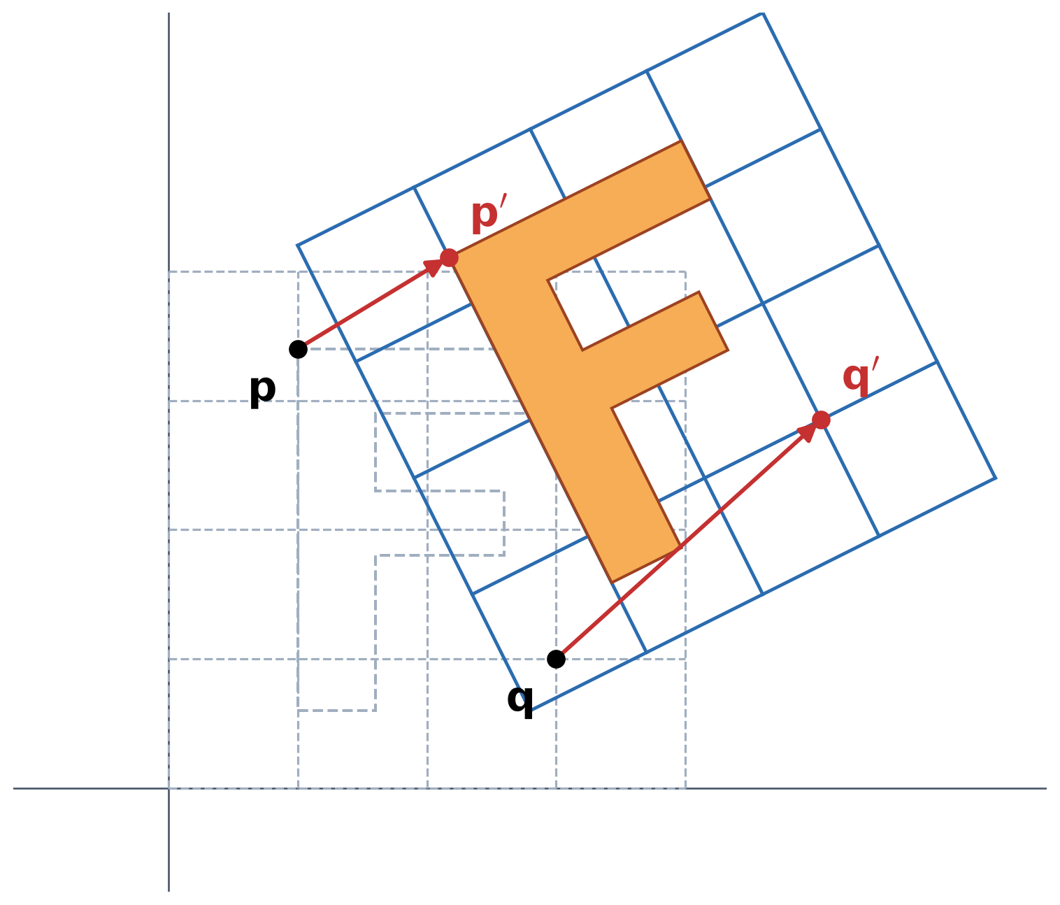
- A transformation \(T\) maps every point \(\mathbf{p} = (x, y)\) to a new point \(\mathbf{p}' = T(\mathbf{p})\).
- Parametric: \(T\) is described by a few numbers (its parameters).
- Global: the same \(T\) applies to every point of the image.
- If \(T\) is linear, it is a matrix: \(\mathbf{p}' = \mathbf{M}\,\mathbf{p}\),
\[ \begin{bmatrix} p'_x \\ p'_y \end{bmatrix} = \underbrace{\begin{bmatrix} m_{11} & m_{12} \\ m_{21} & m_{22} \end{bmatrix}}_{\mathbf{M}} \begin{bmatrix} p_x \\ p_y \end{bmatrix} . \]
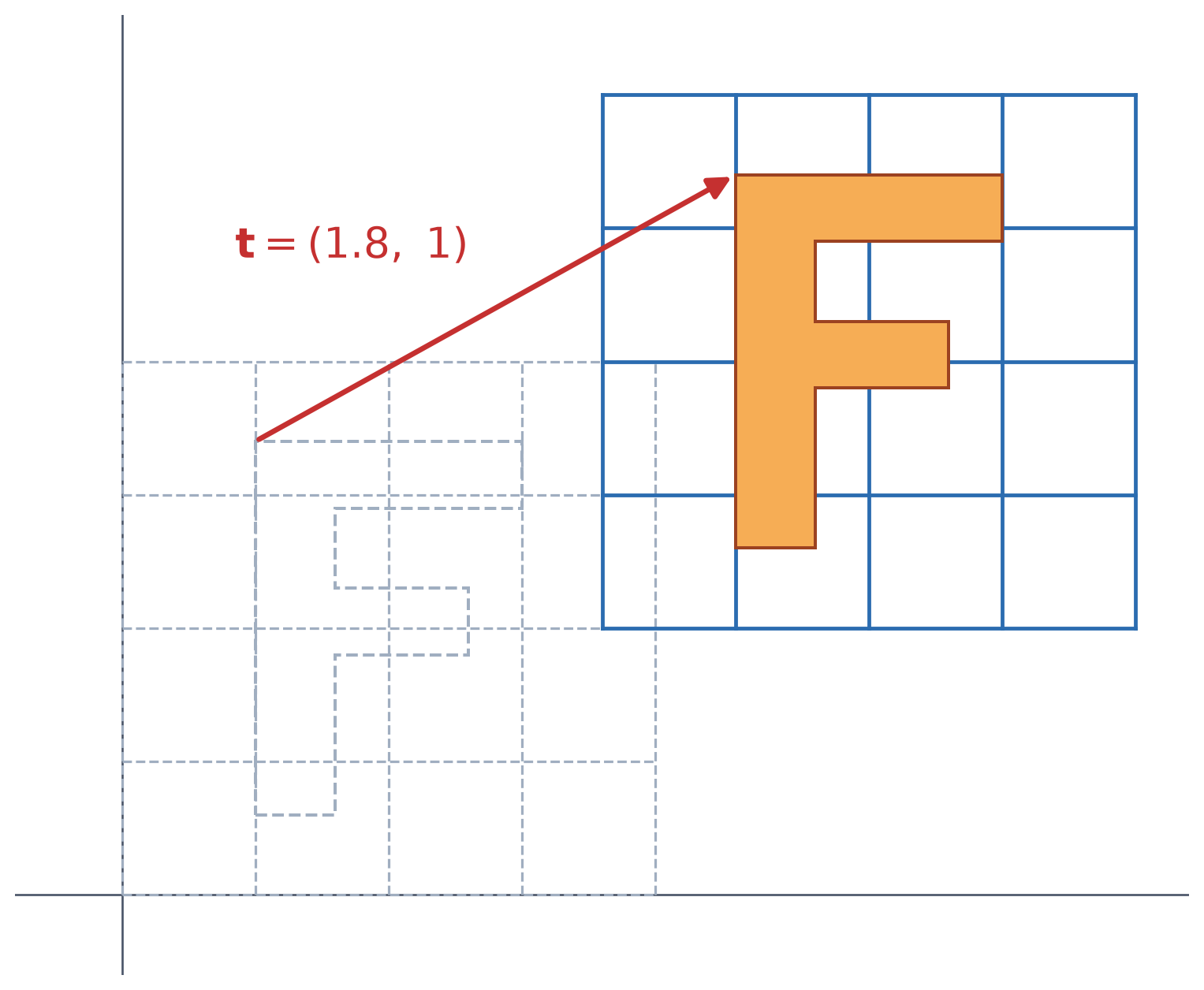
Translation as a Matrix Product
- In Cartesian coordinates, translation is not a matrix product: \[\begin{bmatrix} x' \\ y' \end{bmatrix} = \begin{bmatrix} x \\ y \end{bmatrix} + \begin{bmatrix} t_x \\ t_y \end{bmatrix}\]
- In homogeneous coordinates, it is: \[\begin{bmatrix} x' \\ y' \\ 1 \end{bmatrix} = \begin{bmatrix} 1 & 0 & t_x \\ 0 & 1 & t_y \\ 0 & 0 & 1 \end{bmatrix} \begin{bmatrix} x \\ y \\ 1 \end{bmatrix}\]
- Rotation, scaling, translation, and projection all become matrices, so a sequence of them is one matrix product.
2D Transformation Matrices

| Translation | Uniform scale | Non-uniform scale | Shear | Rotation | |
|---|---|---|---|---|---|
| Cartesian | none: \(\mathbf{p}' = \mathbf{p} + \mathbf{t}\) | \(\begin{bmatrix} s & 0 \\ 0 & s \end{bmatrix}\) | \(\begin{bmatrix} s_x & 0 \\ 0 & s_y \end{bmatrix}\) | \(\begin{bmatrix} 1 & a_x \\ a_y & 1 \end{bmatrix}\) | \(\begin{bmatrix} \cos\theta & -\sin\theta \\ \sin\theta & \cos\theta \end{bmatrix}\) |
| Homogeneous | \(\begin{bmatrix} 1 & 0 & t_x \\ 0 & 1 & t_y \\ 0 & 0 & 1 \end{bmatrix}\) | \(\begin{bmatrix} s & 0 & 0 \\ 0 & s & 0 \\ 0 & 0 & 1 \end{bmatrix}\) | \(\begin{bmatrix} s_x & 0 & 0 \\ 0 & s_y & 0 \\ 0 & 0 & 1 \end{bmatrix}\) | \(\begin{bmatrix} 1 & a_x & 0 \\ a_y & 1 & 0 \\ 0 & 0 & 1 \end{bmatrix}\) | \(\begin{bmatrix} \cos\theta & -\sin\theta & 0 \\ \sin\theta & \cos\theta & 0 \\ 0 & 0 & 1 \end{bmatrix}\) |
- Scale, shear, and rotation are linear: they keep the origin fixed. Translation is not, so it has no \(2\times2\) matrix.
- In homogeneous coordinates, every one of them is a \(3\times3\) matrix.
Composing Transformations
\[\mathbf{R} = \begin{bmatrix} \cos 45^\circ & -\sin 45^\circ & 0 \\ \sin 45^\circ & \cos 45^\circ & 0 \\ 0 & 0 & 1 \end{bmatrix}\qquad\qquad \mathbf{T} = \begin{bmatrix} 1 & 0 & 2.2 \\ 0 & 1 & 0 \\ 0 & 0 & 1 \end{bmatrix}\]
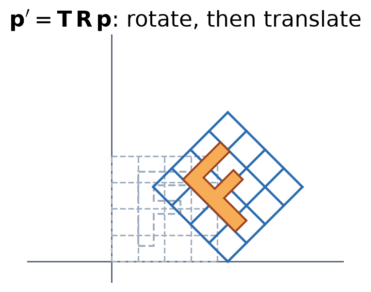
\[\mathbf{T}\,\mathbf{R} = \begin{bmatrix} 0.71 & -0.71 & 2.2 \\ 0.71 & 0.71 & 0 \\ 0 & 0 & 1 \end{bmatrix}\]
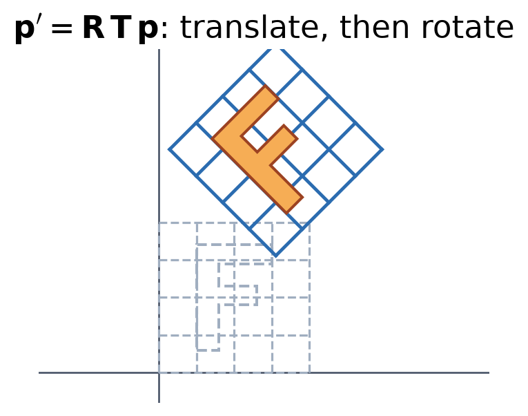
\[\mathbf{R}\,\mathbf{T} = \begin{bmatrix} 0.71 & -0.71 & 1.56 \\ 0.71 & 0.71 & 1.56 \\ 0 & 0 & 1 \end{bmatrix}\]
- A chain of transformations is one matrix, and the rightmost is applied first. Order matters: \(\mathbf{T}\,\mathbf{R} \neq \mathbf{R}\,\mathbf{T}\).
The 2D Transformation Hierarchy
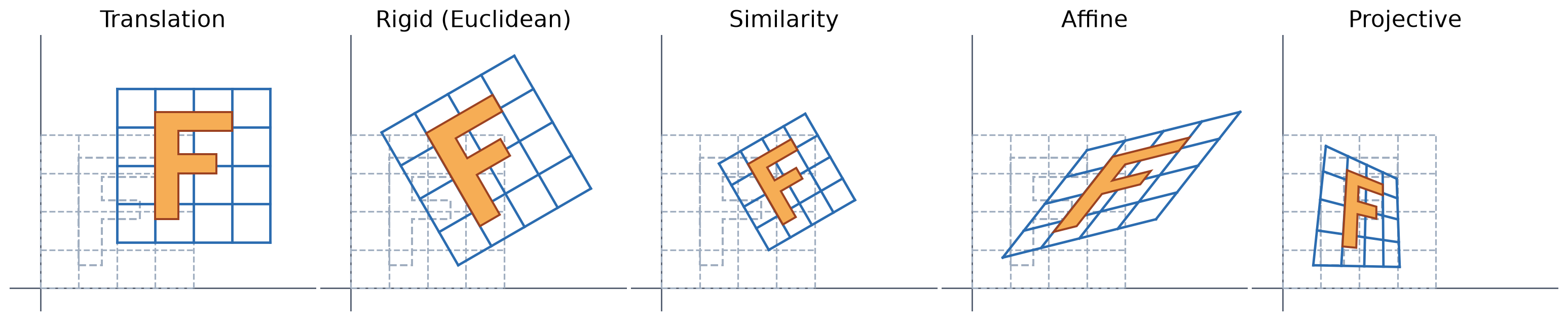
| Transformation | Matrix | DOF | Preserves (and everything below) |
|---|---|---|---|
| Translation | \(\begin{bmatrix} \mathbf{I} & \mathbf{t} \\ \mathbf{0}^{T} & 1 \end{bmatrix}\) | 2 | orientation |
| Rigid (Euclidean) | \(\begin{bmatrix} \mathbf{R} & \mathbf{t} \\ \mathbf{0}^{T} & 1 \end{bmatrix}\) | 3 | lengths |
| Similarity | \(\begin{bmatrix} s\mathbf{R} & \mathbf{t} \\ \mathbf{0}^{T} & 1 \end{bmatrix}\) | 4 | angles |
| Affine | \(\begin{bmatrix} \mathbf{A} & \mathbf{t} \\ \mathbf{0}^{T} & 1 \end{bmatrix}\) | 6 | parallelism |
| Projective | \(\mathbf{H}\) (any invertible \(3\times3\)) | 8 | straight lines |
Affine Transformations
- Any combination of linear transformations and translation: \[\begin{bmatrix} x' \\ y' \\ 1 \end{bmatrix} = \begin{bmatrix} a & b & c \\ d & e & f \\ 0 & 0 & 1 \end{bmatrix} \begin{bmatrix} x \\ y \\ 1 \end{bmatrix}\]
- 6 DOF; the last row is always \([\,0\ \ 0\ \ 1\,]\).
- Properties:
- Lines map to lines
- Parallel lines stay parallel
- Ratios along a line are kept (a midpoint stays a midpoint)
- Closed under composition

Projective Transformations (Homographies)
- A general \(3\times3\) matrix in homogeneous coordinates: \[\begin{bmatrix} x' \\ y' \\ w' \end{bmatrix} = \begin{bmatrix} h_{11} & h_{12} & h_{13} \\ h_{21} & h_{22} & h_{23} \\ h_{31} & h_{32} & h_{33} \end{bmatrix} \begin{bmatrix} x \\ y \\ 1 \end{bmatrix}\]
- Divide by \(w'\) to get the point: a projective warp.
- 8 DOF: \(\mathbf{H}\) is defined only up to scale.
- Properties:
- Lines map to lines
- Parallel lines do not stay parallel
- Ratios are not kept
- Closed under composition

Cameras Are Projective Transformation Machines
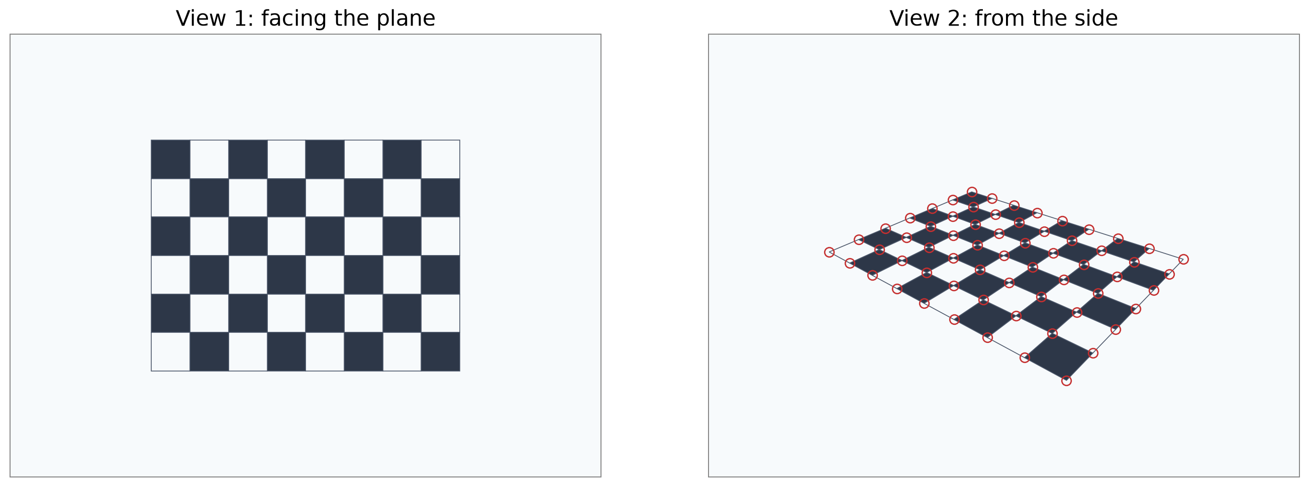
- A camera maps a plane in the world to the image by a homography, so two views of the same plane are related by a homography \(\mathbf{H}\).
- This works only because the scene is flat: for a 3D scene, points at different depths shift by different amounts between views, so no single \(\mathbf{H}\) relates them.
3D Rotation and Translation
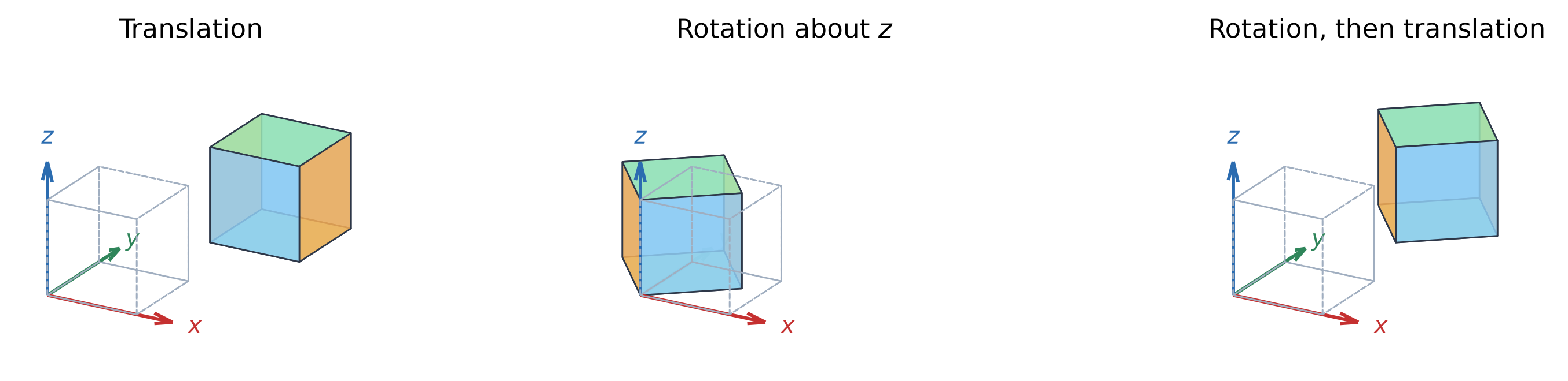
| Translation | Rotation | Rotation + translation (rigid) | |
|---|---|---|---|
| Cartesian | none: \(\mathbf{X}' = \mathbf{X} + \mathbf{t}\) | \(\mathbf{X}' = \mathbf{R}\,\mathbf{X}\) | \(\mathbf{X}' = \mathbf{R}\,\mathbf{X} + \mathbf{t}\) |
| Homogeneous (\(4\times4\)) | \(\begin{bmatrix} \mathbf{I} & \mathbf{t} \\ \mathbf{0}^{T} & 1 \end{bmatrix}\) | \(\begin{bmatrix} \mathbf{R} & \mathbf{0} \\ \mathbf{0}^{T} & 1 \end{bmatrix}\) | \(\begin{bmatrix} \mathbf{R} & \mathbf{t} \\ \mathbf{0}^{T} & 1 \end{bmatrix}\) |
- \(\mathbf{R}\) is a \(3\times3\) rotation; e.g., about \(z\) it is the 2D rotation with a 1 added: \(\;\mathbf{R}_z(\theta) = \begin{bmatrix} \cos\theta & -\sin\theta & 0 \\ \sin\theta & \cos\theta & 0 \\ 0 & 0 & 1 \end{bmatrix}\)
- Every 3D rotation has \(\mathbf{R}^{T}\mathbf{R} = \mathbf{I}\), \(\det\mathbf{R} = 1\), and 3 DOF (e.g., \(\mathbf{R} = \mathbf{R}_z\mathbf{R}_y\mathbf{R}_x\)). A rigid transformation has 6 DOF (\(3 + 3\)).
Changing Coordinate Frames
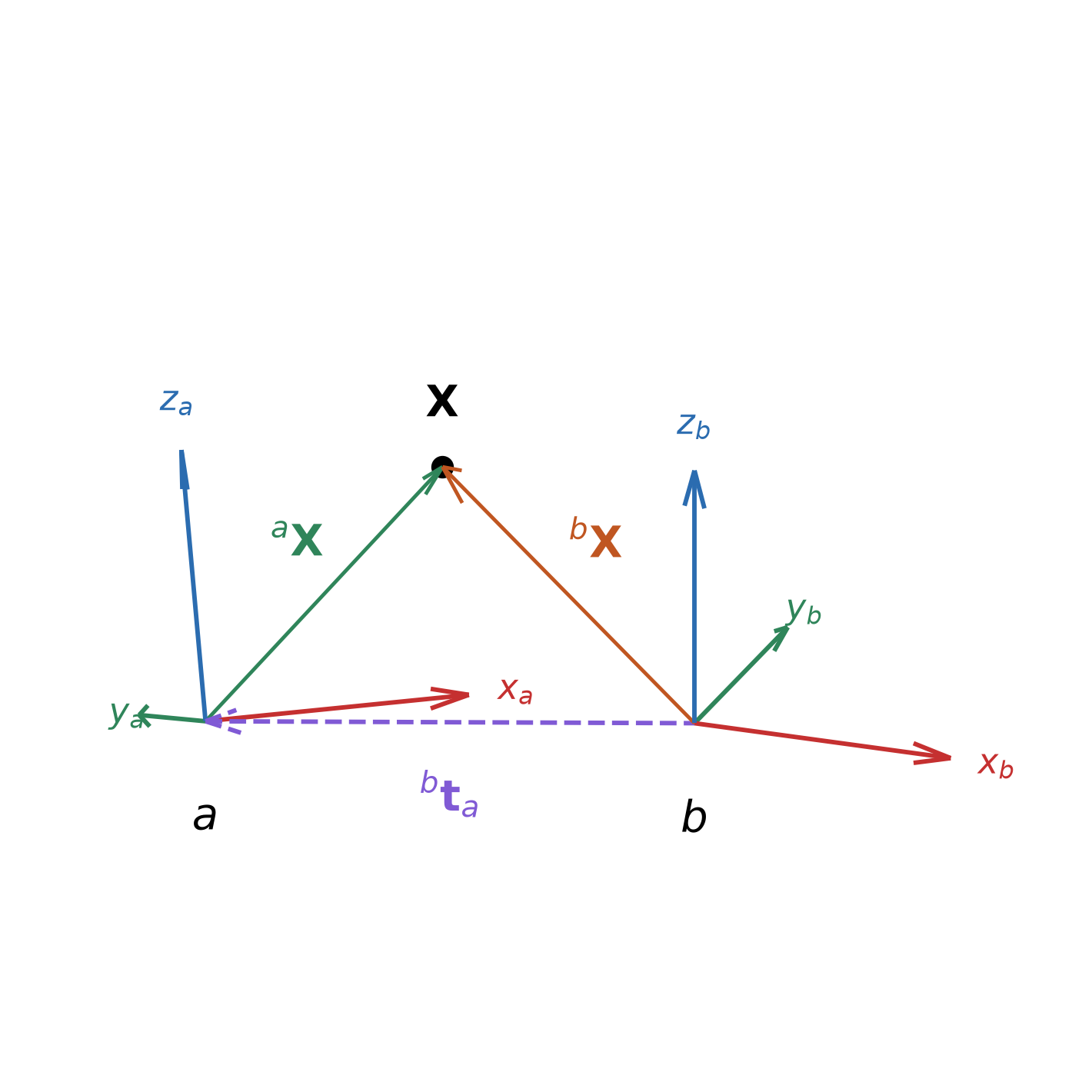
- The same \([\,\mathbf{R} \mid \mathbf{t}\,]\) can move a point within one frame, or change frames (i.e., give the coordinates of one fixed point in another frame): \[
{}^{b}\mathbf{X} = {}^{b}\mathbf{R}_{a}\;{}^{a}\mathbf{X} + {}^{b}\mathbf{t}_{a}
\qquad
{}^{b}\mathbf{T}_{a} = \begin{bmatrix} {}^{b}\mathbf{R}_{a} & {}^{b}\mathbf{t}_{a} \\ \mathbf{0}^{T} & 1 \end{bmatrix}
\]
- Columns of \({}^{b}\mathbf{R}_{a}\): the axes of \(a\) in frame \(b\).
- \({}^{b}\mathbf{t}_{a}\): the origin of \(a\) in frame \(b\).
- Inverse: \[{}^{a}\mathbf{T}_{b} = \left({}^{b}\mathbf{T}_{a}\right)^{-1} = \begin{bmatrix} {}^{b}\mathbf{R}_{a}^{T} & -{}^{b}\mathbf{R}_{a}^{T}\,{}^{b}\mathbf{t}_{a} \\ \mathbf{0}^{T} & 1 \end{bmatrix}\]
- Composition: \({}^{c}\mathbf{T}_{a} = {}^{c}\mathbf{T}_{b}\;{}^{b}\mathbf{T}_{a}\) (matching inner frames cancel).
Camera Model: From a World Point to a Pixel
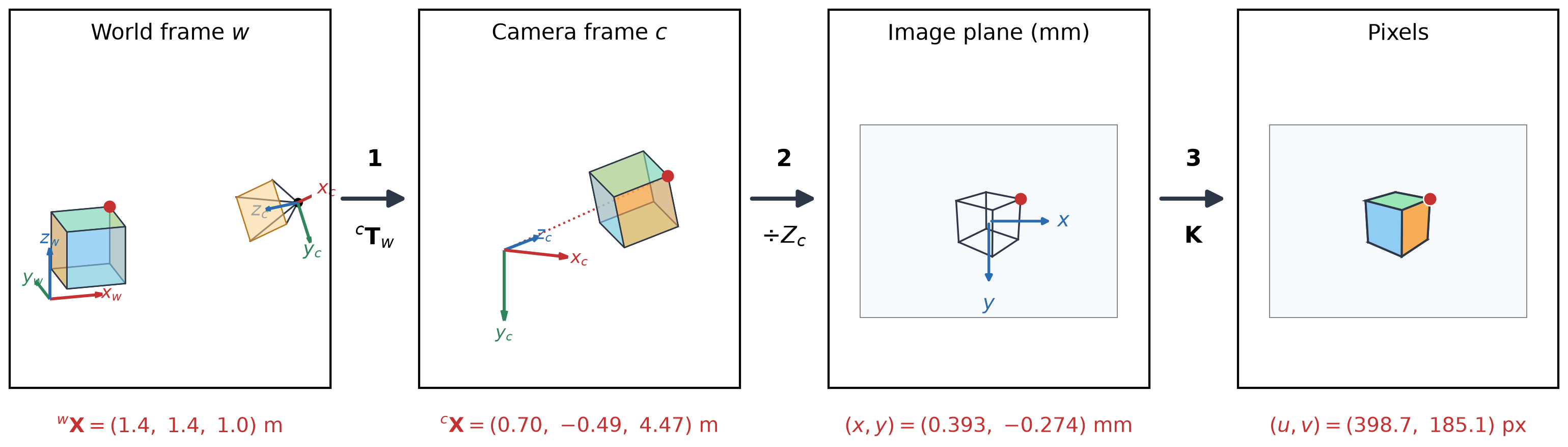
| 1. Extrinsics | 2. Perspective projection | 3. Intrinsics |
|---|---|---|
| world frame \(\to\) camera frame | camera frame \(\to\) image plane | image plane \(\to\) pixels |
Each step is a matrix in homogeneous coordinates, so the whole camera model is one matrix.
Step 1 — World to Camera (Extrinsics)
- Points are given in a world frame \(w\); projection needs them in the camera frame \(c\): \[{}^{c}\mathbf{X} = {}^{c}\mathbf{R}_{w}\;{}^{w}\mathbf{X} + {}^{c}\mathbf{t}_{w} \qquad {}^{c}\mathbf{T}_{w} = \begin{bmatrix} {}^{c}\mathbf{R}_{w} & {}^{c}\mathbf{t}_{w} \\ \mathbf{0}^{T} & 1 \end{bmatrix}\]
- The extrinsic matrix is the top three rows of \({}^{c}\mathbf{T}_{w}\): \(\big[\,{}^{c}\mathbf{R}_{w} \mid {}^{c}\mathbf{t}_{w}\,\big]\) (\(3\times4\)).
- The camera center \({}^{w}\mathbf{C}\) maps to \({}^{c}\mathbf{X} = \mathbf{0}\), so \({}^{c}\mathbf{t}_{w} = -\,{}^{c}\mathbf{R}_{w}\,{}^{w}\mathbf{C}\).
- 6 DOF: camera position is 3 and its orientation is 3.
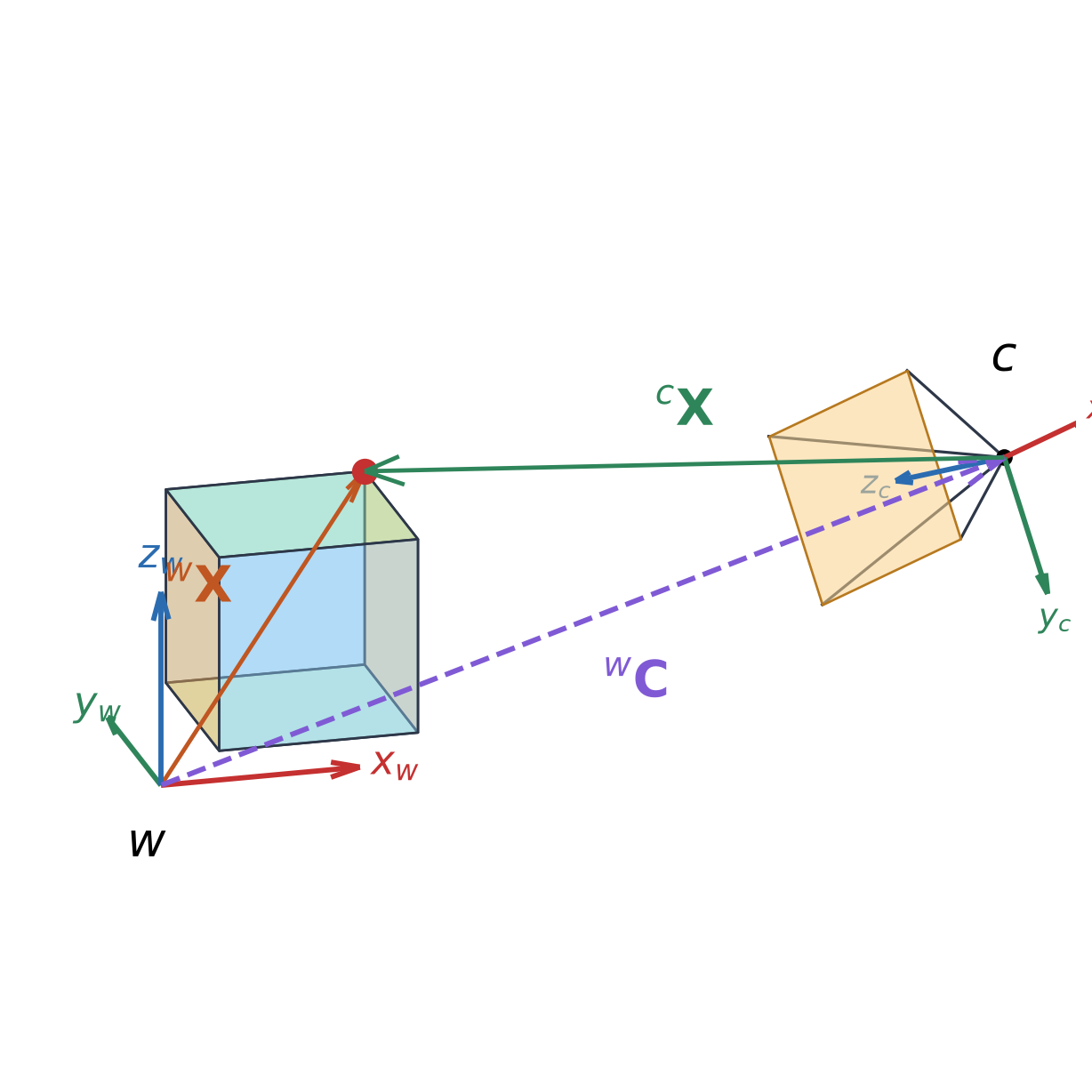
- Example: \({}^{w}\mathbf{C} = ({3.6},\ {-2.4},\ {2.2})\), and the red corner \({}^{w}\mathbf{X} = ({1.4},\ {1.4},\ {1.0})\) becomes \({}^{c}\mathbf{X} = ({0.70},\ {-0.49},\ {4.47})\).
Step 2 — Camera to Image Plane (Projection)
- With \({}^{c}\mathbf{X} = (X_c, Y_c, Z_c)\), perspective projection \(x = f X_c / Z_c\), \(\ y = f Y_c / Z_c\) is a matrix product in homogeneous coordinates: \[Z_c \begin{bmatrix} x \\ y \\ 1 \end{bmatrix} = \begin{bmatrix} f X_c \\ f Y_c \\ Z_c \end{bmatrix} = \begin{bmatrix} f & 0 & 0 & 0 \\ 0 & f & 0 & 0 \\ 0 & 0 & 1 & 0 \end{bmatrix} \begin{bmatrix} X_c \\ Y_c \\ Z_c \\ 1 \end{bmatrix}\]
- The homogeneous scale is the depth \(\lambda = Z_c\): we divide by it only at the end.
- All points on a ray through the camera center give the same \((x, y)\): depth is lost.

- Example (\(f = 2.5\) mm): \({}^{c}\mathbf{X} = ({0.70},\ {-0.49},\ {4.47})\) m \(\Rightarrow\) \((x, y) = ({0.393},\ {-0.274})\) mm, with \(\lambda = 4.47\).
Step 3 — Image Plane to Pixels (Intrinsics)
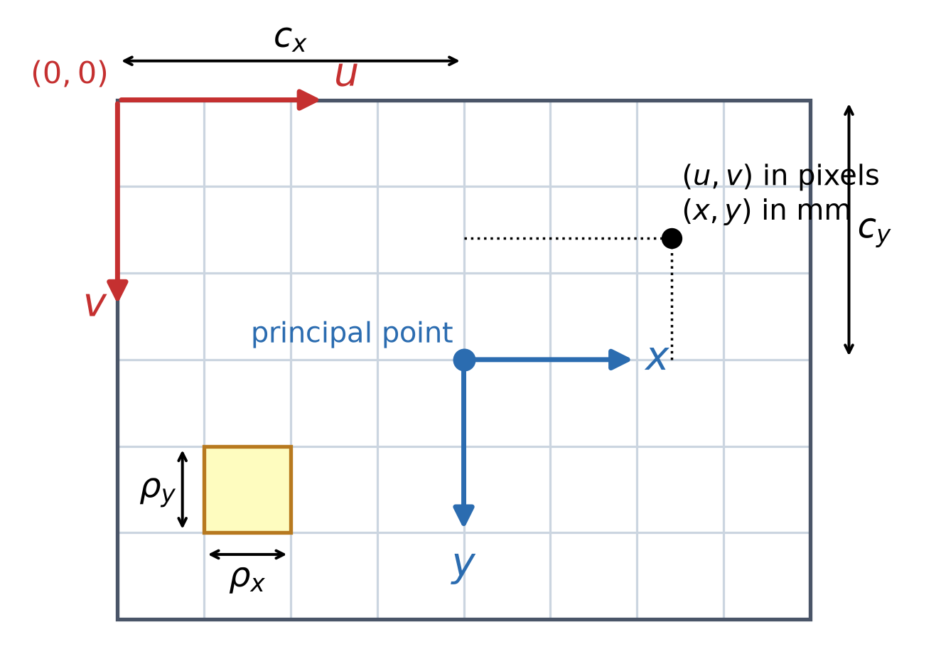
- \((x, y)\) are in mm, with the origin at the principal point.
- Pixel coordinates \((u, v)\) start at the top-left pixel.
- With pixel size \(\rho_x \times \rho_y\) (mm) and the principal point at pixel \((c_x, c_y)\): \[u = \frac{x}{\rho_x} + c_x, \qquad v = \frac{y}{\rho_y} + c_y\]
- As a matrix in homogeneous coordinates: \[\begin{bmatrix} u \\ v \\ 1 \end{bmatrix} = \begin{bmatrix} \tfrac{1}{\rho_x} & 0 & c_x \\ 0 & \tfrac{1}{\rho_y} & c_y \\ 0 & 0 & 1 \end{bmatrix} \begin{bmatrix} x \\ y \\ 1 \end{bmatrix}\]
Intrinsics in Action
- \(f_x, f_y\): focal length in pixels, i.e., zoom; \(f_x \neq f_y\) if pixels are not square.
- \(c_x, c_y\): principal point in pixels, usually near the image center.
- \(s\): skew; \(s = 0\) for almost all modern cameras.
- 5 DOF. The animation changes one parameter at a time, with the camera fixed.

Extrinsics in Action

- \(\mathbf{K}\) is fixed: every change in the image comes from the extrinsic matrix \(\big[\,{}^{c}\mathbf{R}_{w} \mid {}^{c}\mathbf{t}_{w}\,\big]\), shown on the right.
Projecting Points by Hand
K = np.array([[500.0, 0.0, 320.0], [0.0, 500.0, 240.0], [0.0, 0.0, 1.0]]) # intrinsics
rvec = np.array([0.3, -0.4, 0.1])
R_c_w, _ = cv2.Rodrigues(rvec) # extrinsics rotation
t_c_w = np.array([[-0.4], [-0.3], [3.0]]) # extrinsics translation
P = K @ np.hstack([R_c_w, t_c_w]) # camera matrix
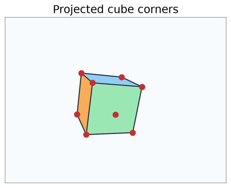
X_w = np.array([[x, y, z] for x in (0, 1) for y in (0, 1) for z in (0, 1)], dtype=float) # cube corners
X_w_h = np.hstack([X_w, np.ones((len(X_w), 1))]) # homogeneous coordinates
x = (P @ X_w_h.T).T # projection (lambda * u, lambda * v, lambda)
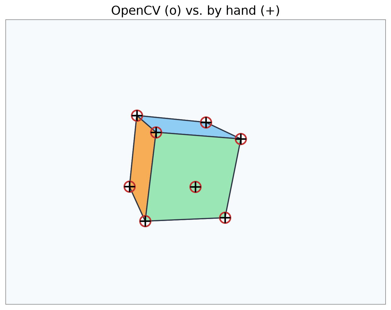
uv = x[:, :2] / x[:, 2:] # pixel coordinates (u, v)rvec: the rotation as a 3-vector (axis \(\times\) angle);cv2.Rodriguesturns it into \({}^{c}\mathbf{R}_{w}\).P\(= \mathbf{K}\,[\,{}^{c}\mathbf{R}_{w} \mid {}^{c}\mathbf{t}_{w}\,]\).X_w_hholds the corners as homogeneous rows.- Each row of
xis \(\lambda\,(u, v, 1)\) with \(\lambda = Z_c\); dividing by it givesuv.
Projecting Points with OpenCV
projectPointstakes the rotation asrvecand applies \(\mathbf{K}\,[\,{}^{c}\mathbf{R}_{w} \mid {}^{c}\mathbf{t}_{w}\,]\) internally.- It returns an \((N, 1, 2)\) array;
reshape(-1, 2)gives \(N \times 2\) pixel coordinates. - The last argument is the lens distortion model:
Nonehere.- We will cover it in the camera calibration lecture.