Lecture 12 — Camera Calibration

Lecture 12

Kaveh Fathian

Computer Science Department, Colorado School of Mines

Learning Objectives

By the end of this lecture, you should be able to:

  • Explain what geometric calibration estimates: the intrinsic matrix, the lens distortion, and the target poses.
  • Calibrate a camera linearly from a known 3D target, and recover \(\mathbf{K}\), \({}^{c}\mathbf{R}_{w}\), and \({}^{c}\mathbf{t}_{w}\) from the camera matrix.
  • Describe the reprojection error and the radial–tangential, fisheye, and omnidirectional lens models.
  • Calibrate a camera with a checkerboard in OpenCV, and undistort its images.
  • Collect useful calibration images, and check the result with per-view reprojection errors.

What Does It Mean to Calibrate a Camera?

  • To calibrate is to estimate the parameters of a camera model from measurements. There are many kinds:
    • Radiometric: pixel value vs. scene brightness.
    • Color: sensor response vs. true color.
    • Noise: sensor noise level and pattern.
    • Lens aberration: blur, vignetting, chromatic effects.
    • Geometric: where each pixel looks in 3D.
  • This lecture covers geometric calibration. It estimates:
    • The intrinsic matrix \(\mathbf{K}\)
    • The lens distortion coefficients
    • The pose of the target in each image

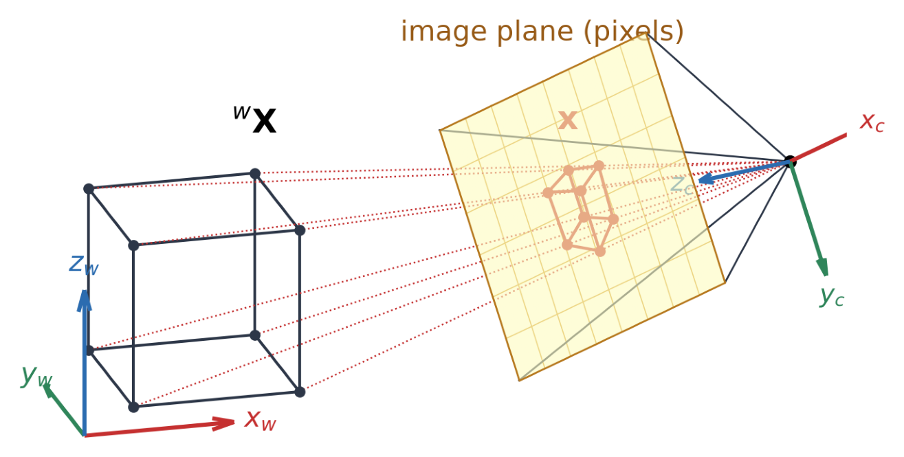
\[ \underbrace{\lambda}_{\text{depth } Z_c}\, \underbrace{\mathbf{x}}_{\substack{\text{pixel}\\ (u,\,v,\,1)}} = \overbrace{ \underbrace{\color{#c53030}{\mathbf{K}}}_{\substack{\text{intrinsic}\\ \text{matrix}}}\; \underbrace{\big[\,{}^{c}\mathbf{R}_{w} \mid {}^{c}\mathbf{t}_{w}\,\big]}_{\substack{\text{extrinsic}\\ \text{matrix}}} }^{\mathbf{P}:\ \text{camera matrix}}\; \underbrace{{}^{w}\mathbf{X}}_{\substack{\text{world point}\\ (X,\,Y,\,Z,\,1)}} \]

Problems Based on Camera Model

\[\lambda\,\mathbf{x} = \mathbf{K}\,\big[\,{}^{c}\mathbf{R}_{w} \mid {}^{c}\mathbf{t}_{w}\,\big]\;{}^{w}\mathbf{X}\]

Which quantities are known and which are unknown defines the problem:

Problem Pixels \(\mathbf{x}\) Intrinsics \(\mathbf{K}\) Extrinsics \({}^{c}\mathbf{R}_{w},\ {}^{c}\mathbf{t}_{w}\) 3D points \({}^{w}\mathbf{X}\)
Projection (simulate a camera) unknown known known known
Camera calibration known unknown unknown known
Two-view geometry known known unknown unknown
Triangulation known known known unknown
  • Calibration is usually done once per camera and lens setting. The estimated/known \(\mathbf{K}\) and distortion are then used in other problems.
  • Calibration is also called resectioning.

Linear Calibration with a Known 3D Target

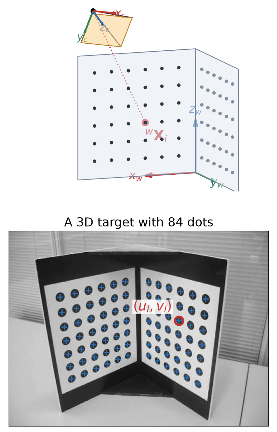
  • Assume given an image of a target whose 3D points \({}^{w}\mathbf{X}_i\) are known, with their pixel positions \((u_i, v_i)\).

  • Unknown: the camera matrix \(\mathbf{P}\), with rows \(\mathbf{p}_1^{T}, \mathbf{p}_2^{T}, \mathbf{p}_3^{T}\).

  • From camera model \(\lambda\,\begin{bmatrix} u_i \\ v_i \\ 1 \end{bmatrix} = \begin{bmatrix} \mathbf{p}_1^{T} \\ \mathbf{p}_2^{T} \\ \mathbf{p}_3^{T} \end{bmatrix}\,{}^{w}\mathbf{X}_i,\) we have: \[\lambda u_i = \mathbf{p}_1^{T}\,{}^{w}\mathbf{X}_i, \qquad \lambda v_i = \mathbf{p}_2^{T}\,{}^{w}\mathbf{X}_i, \qquad \lambda = \mathbf{p}_3^{T}\,{}^{w}\mathbf{X}_i \]

  • Substituting \(\lambda=\mathbf{p}_3^{T}\,{}^{w}\mathbf{X}_i\) in the first two equations gives two equations per point, both linear in the 12 entries of \(\mathbf{P}\): \[\mathbf{p}_1^{T}\,{}^{w}\mathbf{X}_i - u_i\,\mathbf{p}_3^{T}\,{}^{w}\mathbf{X}_i = 0\] \[\mathbf{p}_2^{T}\,{}^{w}\mathbf{X}_i - v_i\,\mathbf{p}_3^{T}\,{}^{w}\mathbf{X}_i = 0\]
Direct Linear Transform (DLT)

  • Stack the two rows of every point into \(\mathbf{A}\) and solve \(\mathbf{A}\mathbf{p} = \mathbf{0}\) with the SVD: \[\underbrace{\begin{bmatrix} {}^{w}\mathbf{X}_1^{T} & \mathbf{0}^{T} & -u_1\,{}^{w}\mathbf{X}_1^{T} \\ \mathbf{0}^{T} & {}^{w}\mathbf{X}_1^{T} & -v_1\,{}^{w}\mathbf{X}_1^{T} \\ \vdots & \vdots & \vdots \end{bmatrix}}_{\mathbf{A}:\ 2N \times 12} \underbrace{\begin{bmatrix} \mathbf{p}_1 \\ \mathbf{p}_2 \\ \mathbf{p}_3 \end{bmatrix}}_{12 \times 1} = \mathbf{0}\]
  • \(\mathbf{P}\) has 11 DOF and each point gives 2 equations: at least 6 points, not all on one plane.
  • The more points we use, the more robust the solution is to noise as it is averaged out.
  • \(\mathbf{P}\) and \(-\mathbf{P}\) are both solutions; keep the sign that puts the points in front of the camera.
def calibrate_dlt(X_w, uv):
    A = []
    for X, (u, v) in zip(X_w, uv):
        X_h = np.append(X, 1)
        z = np.zeros(4)
        A += [np.r_[X_h, z, -u * X_h],
              np.r_[z, X_h, -v * X_h]]
    _, _, Vt = np.linalg.svd(np.array(A))
    P = Vt[-1].reshape(3, 4)
    if np.linalg.det(P[:, :3]) < 0:
        P = -P
    return P

Example output for the target points of the previous slide:

\[\mathbf{P}_{\text{DLT}} = \begin{bmatrix} -0.487 & 0.221 & -0.202 & 0.483 \\ 0.108 & 0.0902 & -0.514 & 0.395 \\ -0.000563 & -0.000466 & -0.000631 & 0.00157 \end{bmatrix}\]

Least-Squares Review (Supplementary)

  • When we have more equations than unknowns (plus noise), there is no exact solution. Least-squares find the best approximate solution that minimizes the sum of squared errors. There are two cases:

  • Nonhomogeneous \(\mathbf{A}\mathbf{p} = \mathbf{b}\): \[\min_{\mathbf{p}} \|\mathbf{A}\mathbf{p} - \mathbf{b}\|^2 \;\Rightarrow\; \mathbf{p} = (\mathbf{A}^{T}\mathbf{A})^{-1}\mathbf{A}^{T}\mathbf{b}\]

  • Homogeneous \(\mathbf{A}\mathbf{p} = \mathbf{0}\):

    • \(\mathbf{p} = \mathbf{0}\) is trivial, and any scaled solution is a solution, so fix the scale \(\|\mathbf{p}\| = 1\): \[\min_{\|\mathbf{p}\| = 1} \|\mathbf{A}\mathbf{p}\|^2\;\Rightarrow\; \mathbf{p} = \text{last right singular vector of } \mathbf{A}\]
  • Calibration is the homogeneous case: \(\mathbf{P}\) is only defined up to scale.

  • In NumPy:

    • \(\mathbf{A}\mathbf{p} = \mathbf{b} \implies\) p = np.linalg.lstsq(A, b)[0]
    • \(\mathbf{A}\mathbf{p} = \mathbf{0} \implies\) p = np.linalg.svd(A)[2][-1]

Extracting \(\mathbf{K}\), \({}^{c}\mathbf{R}_{w}\), and \({}^{c}\mathbf{t}_{w}\) From \(\mathbf{P}\)

  • The left \(3 \times 3\) block of \(\mathbf{P}\) is \(\mathbf{M} = \mathbf{K}\,{}^{c}\mathbf{R}_{w}\): upper triangular times a rotation.
  • RQ decomposition splits \(\mathbf{M}\) into these two factors (“R” = upper triangular \(\mathbf{K}\), “Q” = rotation \({}^{c}\mathbf{R}_{w}\)). Signs are fixed so \(\mathbf{K}\) has a positive diagonal.
  • With \(\mathbf{p}_4\) the last column of \(\mathbf{P}\): \[{}^{c}\mathbf{t}_{w} = \mathbf{K}^{-1}\,\mathbf{p}_4, \qquad {}^{w}\mathbf{C} = -\mathbf{M}^{-1}\,\mathbf{p}_4\]
  • OpenCV does all of this:
K_est, R_est, C_h, *_ = cv2.decomposeProjectionMatrix(P_dlt)
K_est = K_est / K_est[2, 2]           # K, normalized so that K[2, 2] = 1
C_est = C_h[:3, 0] / C_h[3, 0]        # camera center wC from homogeneous coordinates
t_est = -R_est @ C_est                # ct_w = -cR_w wC

Limits of Linear Calibration

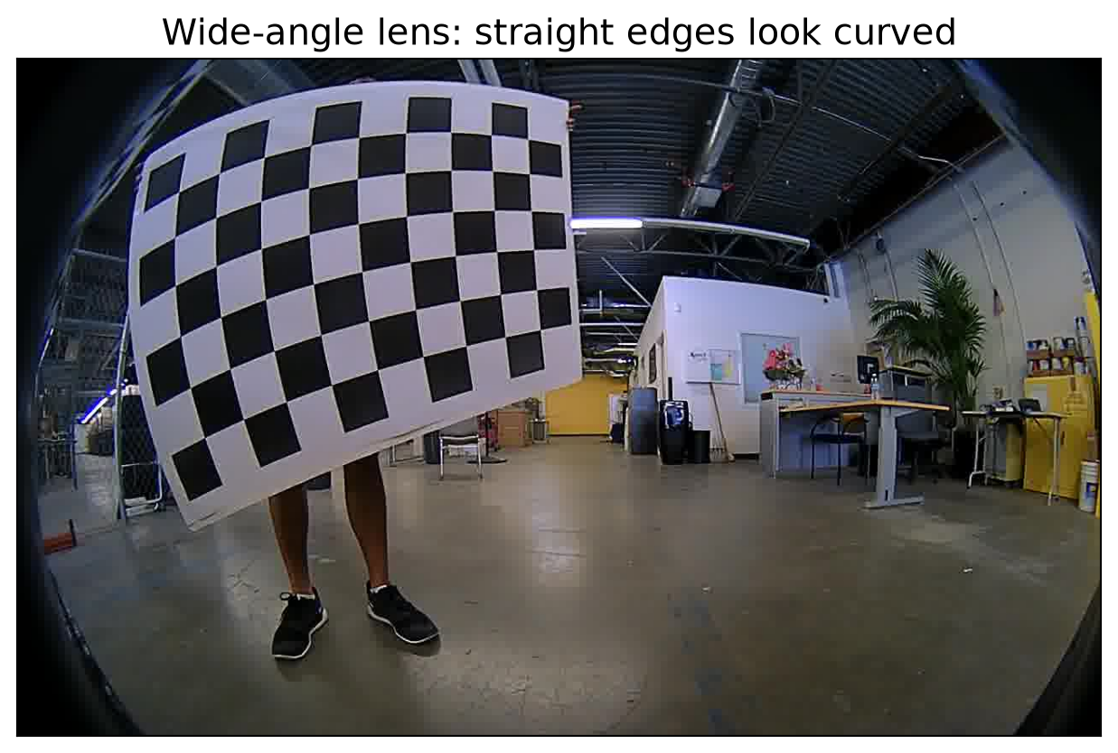
  • No lens distortion. A wide-angle lens bends straight lines, which no \(\mathbf{P}\) can model.
  • Wrong error. It minimizes the algebraic error \(\|\mathbf{A}\mathbf{p}\|\), not the distance in pixels.
  • No constraints. Known facts, such as \(s = 0\), are hard to enforce.
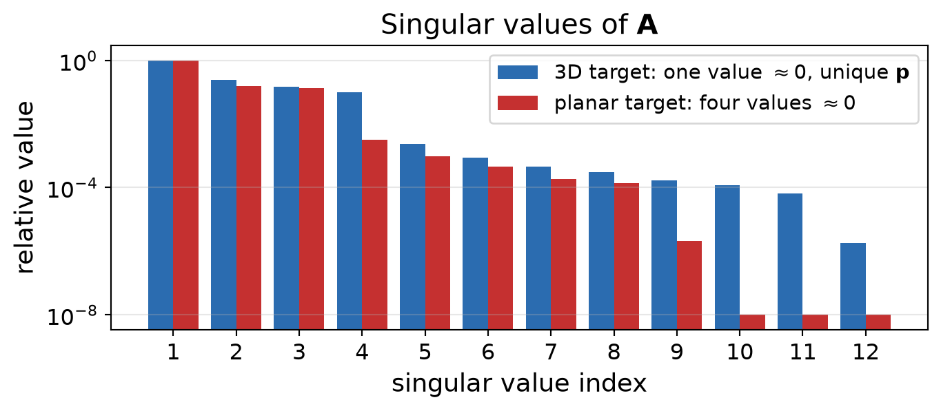
  • Needs a precise 3D target. If all points lie on one plane (\(Z = 0\)), the columns of \(\mathbf{A}\) that multiply \(Z\) are zero, and \(\mathbf{p}\) is not unique (right).
  • In practice: Linear calibration is not used. A linear solution is only the initial guess, which is used in nonlinear optimization to refine all parameters, including lens distortion.
Nonlinear Calibration

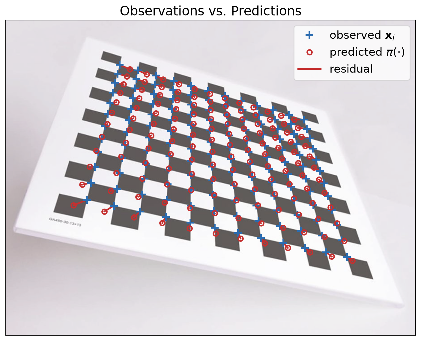
  • Nonlinear calibration compares observed image points \(\mathbf{x}_i = (u_i, v_i)\) with the points predicted by the camera model.
  • The reprojection error is their distance in pixels, summed over all points: \[E = \sum_{i}\Big\|\,\mathbf{x}_{i} - \pi\big(\mathbf{K}, \mathbf{d},\, {}^{c}\mathbf{R}_{w},\, {}^{c}\mathbf{t}_{w},\, {}^{w}\mathbf{X}_i\big)\Big\|^2\]
    • \(\mathbf{d}\): lens distortion coefficients (next slides).
    • \({}^{c}\mathbf{R}_{w}, {}^{c}\mathbf{t}_{w}\): pose of the target (world frame \(w\)) in the camera frame.
    • \(\pi(\cdot)\): the camera model.
  • \(E\) is nonlinear in the parameters. It is minimized by iterative nonlinear least squares (Levenberg–Marquardt), starting from a linear initial guess.
  • In practice, the target is imaged in many views \(j\), and \(E\) sums over all of them: one \(\mathbf{K}\) and \(\mathbf{d}\), plus one pose \({}^{c_j}\mathbf{R}_{w}, {}^{c_j}\mathbf{t}_{w}\) per view.
The Lens Distortion Model

  • Distortion acts on the image coordinates, before \(\mathbf{K}\): \[{}^{c}\mathbf{X} \;\to\; (x, y) = \Big(\tfrac{{}^cX}{{}^cZ}, \tfrac{{}^cY}{{}^cZ}\Big) \;\xrightarrow{\text{distortion}}\; (x_d, y_d) \;\xrightarrow{\;\mathbf{K}\;}\; (u, v)\]

    • \((x, y)\): where an ideal pinhole camera sees the point.
    • \((x_d, y_d)\): where the lens actually puts it.
  • With \(r^2 = x^2 + y^2\) (squared distance from the principal point): \[\begin{aligned} x_d &= \underbrace{\color{#2b6cb0}{x\,(1 + k_1 r^2 + k_2 r^4 + k_3 r^6)}}_{\color{#2b6cb0}{\text{radial}}} + \underbrace{\color{#c05621}{2 p_1 x y + p_2 (r^2 + 2 x^2)}}_{\color{#c05621}{\text{tangential}}} \\ y_d &= \underbrace{\color{#2b6cb0}{y\,(1 + k_1 r^2 + k_2 r^4 + k_3 r^6)}}_{\color{#2b6cb0}{\text{radial}}} + \underbrace{\color{#c05621}{p_1 (r^2 + 2 y^2) + 2 p_2 x y}}_{\color{#c05621}{\text{tangential}}} \end{aligned}\]

  • Pixels: \((u, v, 1)^{T} = \mathbf{K}\,(x_d, y_d, 1)^{T}\), instead of \(\mathbf{K}\,(x, y, 1)^{T}\). This is the camera model \(\pi(\cdot)\) of the previous slide.

Calibration animation

Radial Distortion

  • The radial terms scale \((x, y)\) along its ray from the principal point: \(\begin{bmatrix} x_d \\ y_d \end{bmatrix} = s(r) \begin{bmatrix} x \\ y \end{bmatrix}, \quad s(r) = 1 + k_1 r^2 + k_2 r^4 + k_3 r^6\)
  • Only the distance from the center changes, from \(r\) to \(r_d = \sqrt{x_d^2 + y_d^2} = r\,s(r)\)$
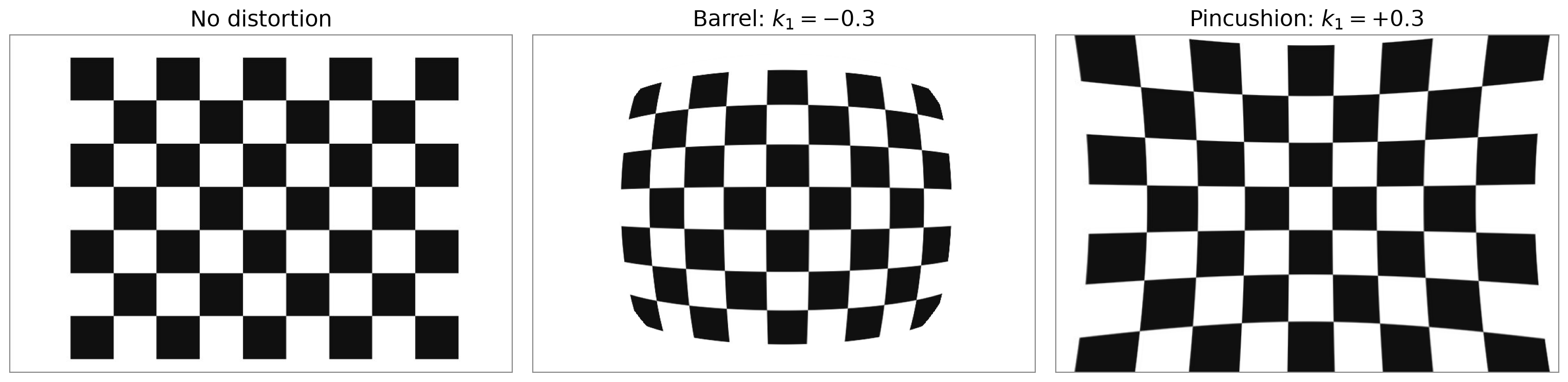
  • Barrel (\(k_1 < 0\), \(s < 1\)): points move toward the center; wide-angle lenses (GoPro, phone ultra-wide).
  • Pincushion (\(k_1 > 0\), \(s > 1\)): points move away from the center; telephoto lenses.
  • Straight lines not through the center become curved. The effect is \(\approx 0\) near the center and grows with \(r\).

Tangential Distortion
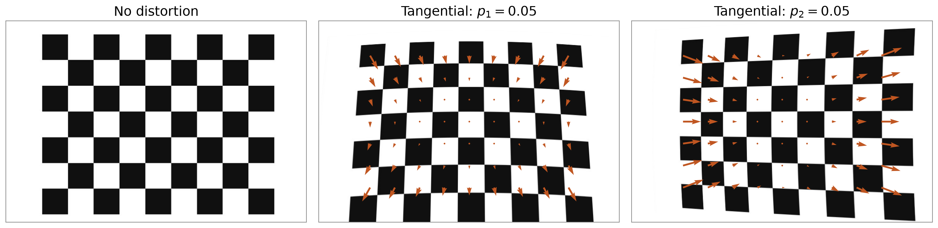
  • The tangential terms shift points sideways, not along their ray from the center: \[x_d = x\,s(r) + \underbrace{\color{#c05621}{2 p_1 x y + p_2 (r^2 + 2 x^2)}}_{\color{#c05621}{\Delta x}}, \qquad y_d = y\,s(r) + \underbrace{\color{#c05621}{p_1 (r^2 + 2 y^2) + 2 p_2 x y}}_{\color{#c05621}{\Delta y}}\]
  • Cause: lens elements slightly tilted or off-center relative to the sensor.
  • Usually small.

Wide Lenses: Fisheye and Omnidirectional

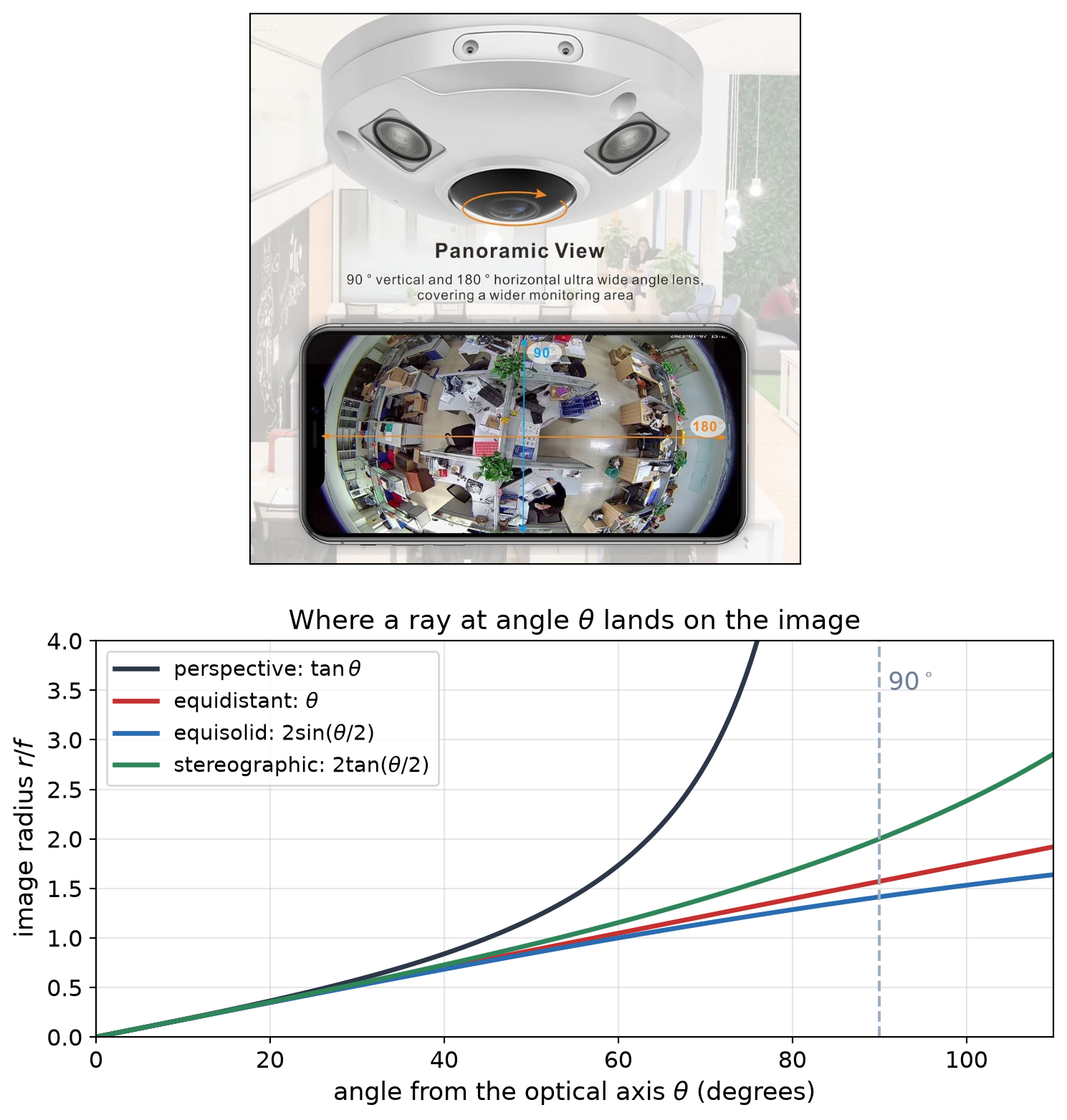
  • A pinhole maps a ray at angle \(\theta\) from the optical axis to radius \(r = f \tan\theta\), which grows to infinity at \(90^\circ\).
  • Fisheye lenses use a different mapping, close to \(r = f\,\theta\), so they can see \(180^\circ\) or more.
    • OpenCV cv2.fisheye: \(\theta_d = \theta\,(1 + k_1\theta^2 + k_2\theta^4 + k_3\theta^6 + k_4\theta^8)\)
  • Omnidirectional cameras: field of view \(\geq 180^\circ\), or a curved mirror in front of the lens.
    • OpenCV cv2.omnidir unified sphere model, or Scaramuzza’s polynomial model (OCamCalib).
  • Rule of thumb: radial–tangential up to a field of view (FOV) of about \(100^\circ\)–\(120^\circ\), i.e., \(\theta\) up to \(50^\circ\)–\(60^\circ\) at the image edge; beyond that, fisheye or omnidirectional.
Common Calibration Targets
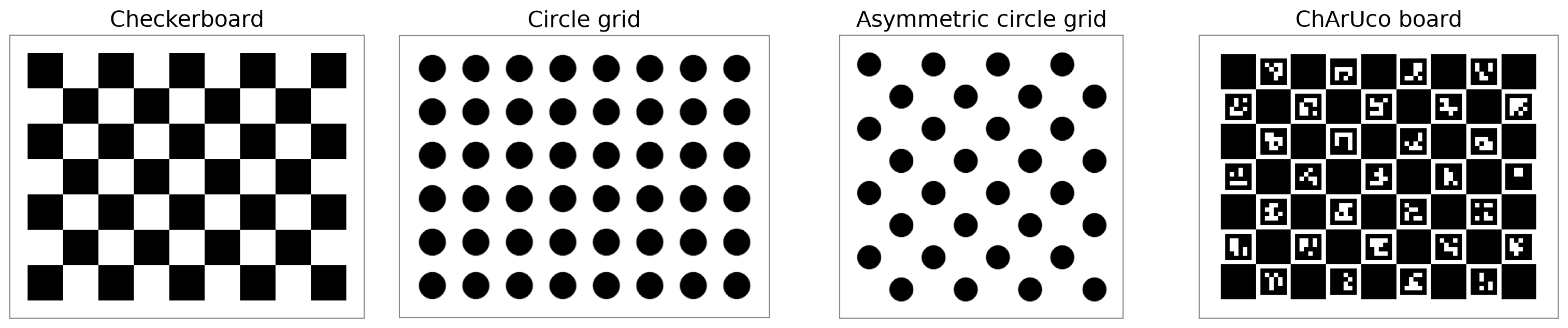
Target OpenCV detector Strengths Weaknesses
Checkerboard findChessboardCorners Simple; accurate corners (sub-pixel) The whole board must be visible
Circle grids findCirclesGrid Robust to blur and noise Circle centers shift slightly under perspective
ChArUco cv2.aruco.CharucoDetector Each corner is identified by its markers: partial and occluded views still work Must be printed exactly to spec
  • ChArUco makes it easy to cover image corners, where distortion is largest, because the board may be partly outside the image.
  • You must know/measure the exact size of the squares/markers in the target to get the correct scale for translation.

Calibration Example in OpenCV
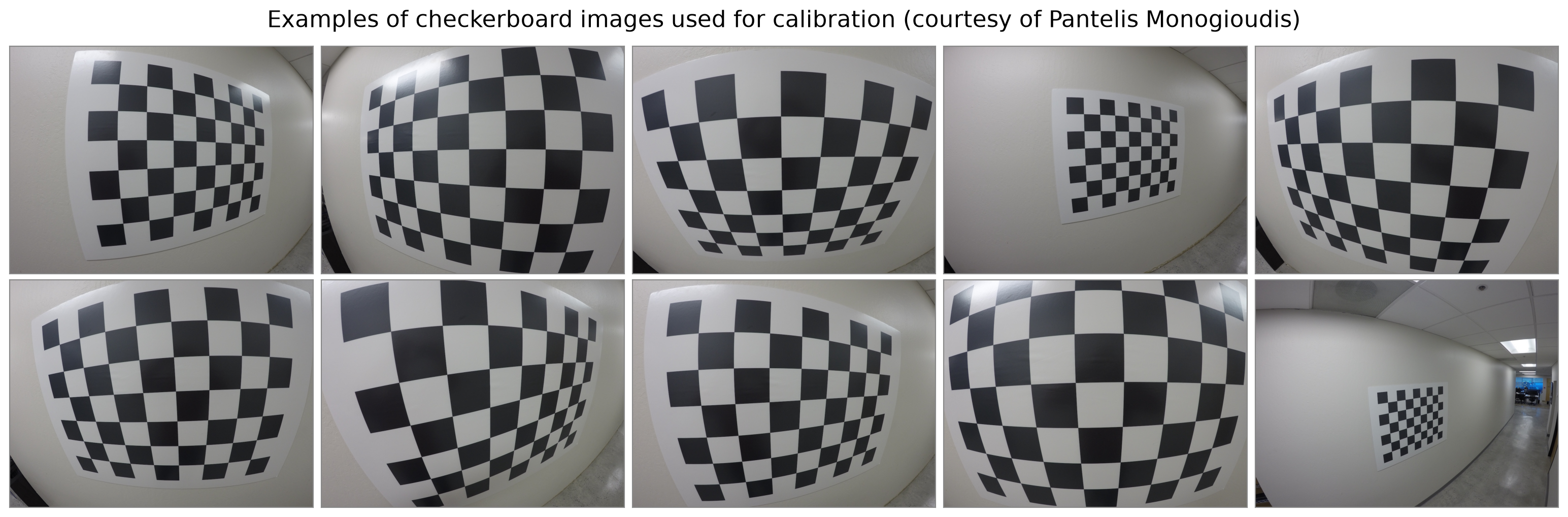
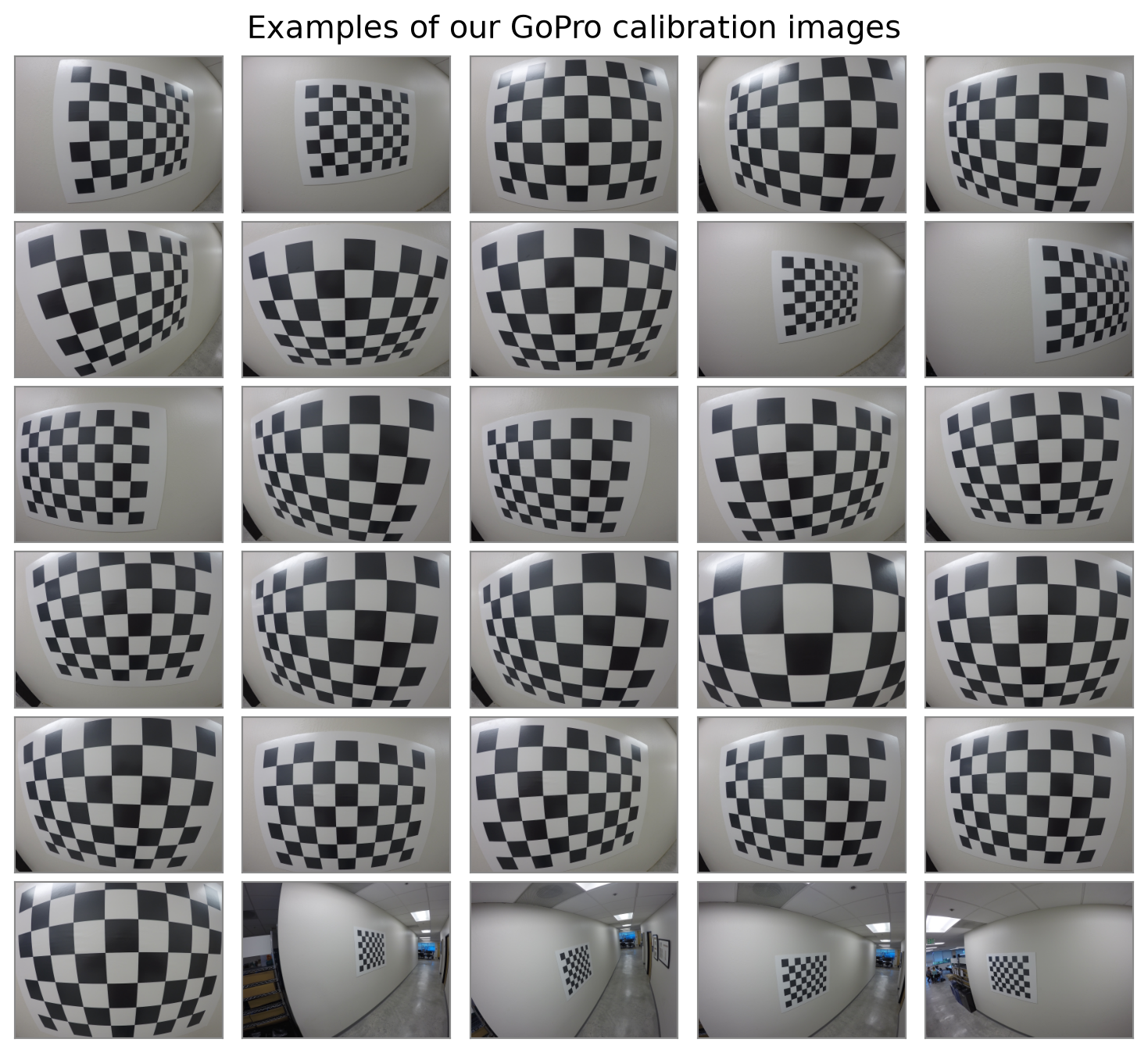
  • \(35\) images from a GoPro camera with a wide-angle lens, \(1280 × 960\) pixels.
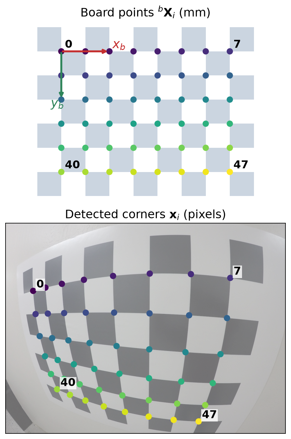
  • Checkerboard with \(9×7\) squares, so \(8×6=48\) inner corners.
  • Square size: \(80\,\text{mm}\).

Step 1: Detect the Corners

img = cv2.imread(str(calib_dir / "GOPR0046.jpg"))
gray = cv2.cvtColor(img, cv2.COLOR_BGR2GRAY)
pattern = (8, 6)  # inner corners per row, per column
found, corners = cv2.findChessboardCorners(gray, pattern)

criteria = (cv2.TERM_CRITERIA_EPS
            + cv2.TERM_CRITERIA_MAX_ITER, 30, 1e-3)
corners_sub = cv2.cornerSubPix(gray, corners.copy(),
                               (11, 11), (-1, -1), criteria)
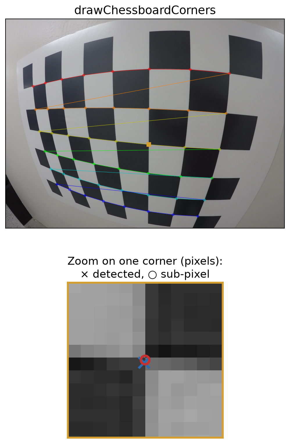
  • corners: the 48 corner pixels, ordered row by row, starting at one end of the board.
  • cornerSubPix refines each corner to sub-pixel accuracy using the image gradients in an \(11 \times 11\) window. It works in place, hence the .copy() here.
  • If found is False, skip the image: the board was not fully visible.
Step 2: Match Corners to Board Points

square = 80.0  # mm 
objp = np.zeros((pattern[0] * pattern[1], 3), np.float32)
objp[:, :2] = np.mgrid[0:8, 0:6].T.reshape(-1, 2) * square

obj_points, img_points = [], []
for path in calib_files:
    gray = cv2.imread(str(path), cv2.IMREAD_GRAYSCALE)
    found, corners = cv2.findChessboardCorners(gray,
                                               pattern)
    if not found:
        continue
    corners = cv2.cornerSubPix(gray, corners, (11, 11),
                               (-1, -1), criteria)
    obj_points.append(objp)
    img_points.append(corners)
  • objp holds the corners \({}^{b}\mathbf{X}_i = (X, Y, 0)\) in the board frame \(b\), in the same order as the detected corners.
  • The board frame moves with the board, so objp is the same for every view.

Step 3: Calibrate

rms, K, dist, rvecs, tvecs = cv2.calibrateCamera(
    obj_points, img_points, image_size, None, None)
  • Inside: a linear initial guess (Zhang’s method), then Levenberg–Marquardt on the reprojection error.
  • rms \(=\) 0.824 px: the RMS reprojection error over all 35 views.
  • K:

\[\mathbf{K} = \begin{bmatrix} 560 & 0 & 651.1 \\ 0 & 561.1 & 498.9 \\ 0 & 0 & 1 \end{bmatrix}\]

  • dist \(= (k_1, k_2, p_1, p_2, k_3)\):

\[(-0.2326,\ 0.0615,\ -0.00003,\ 0.00006,\ -0.0075)\]

  • \(k_1 = -0.23 < 0\): strong barrel distortion, as expected for a GoPro.
  • Horizontal field of view: \(2\arctan\big(\tfrac{W}{2 f_x}\big) = 98^\circ\).
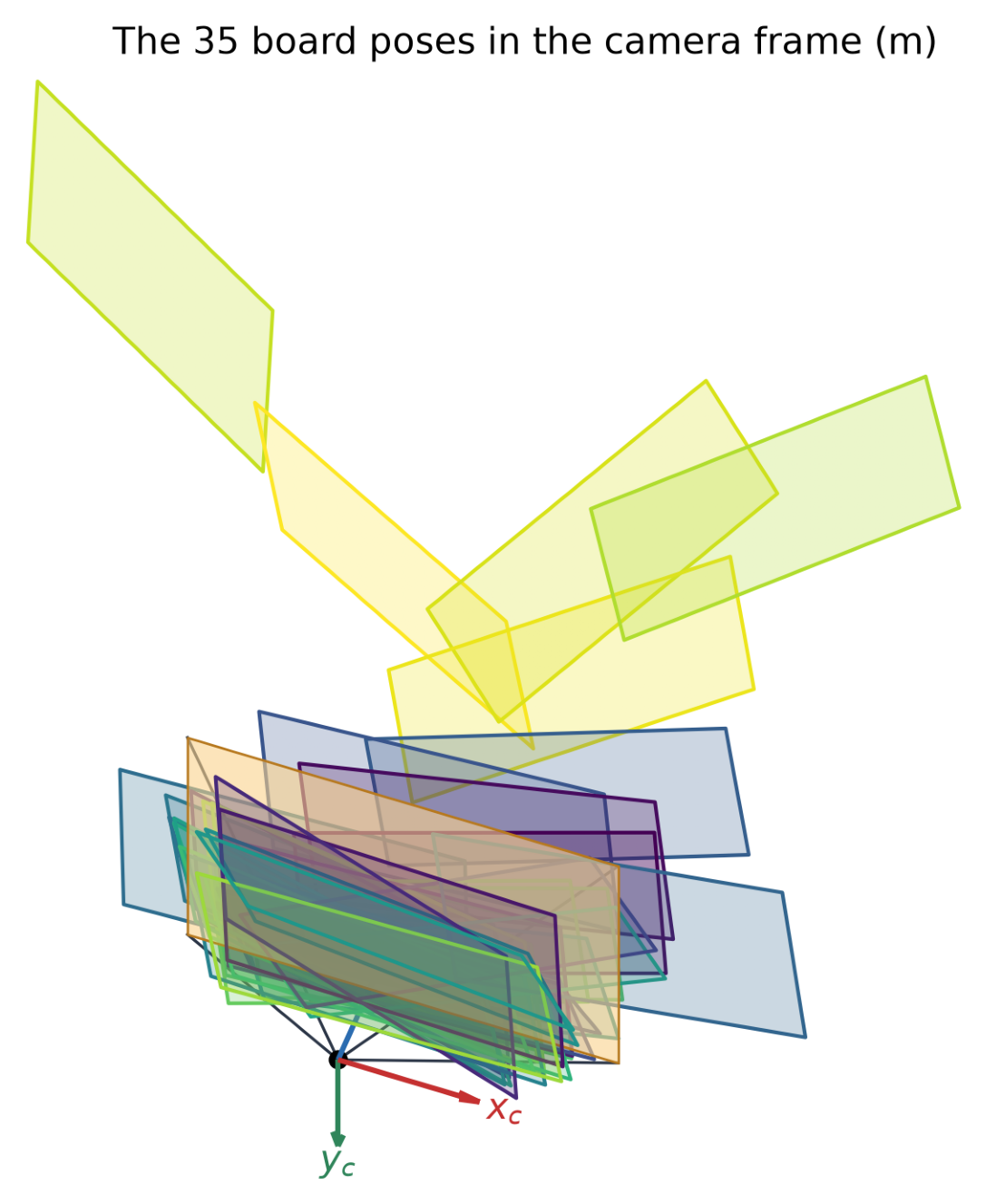
  • rvecs, tvecs: 35 board poses, one per view (next slide).

What Calibration Returns

Output Meaning
K Intrinsic matrix \(\mathbf{K}\): \(f_x, f_y, c_x, c_y\) (skew fixed to 0)
dist Distortion \(\mathbf{d} = (k_1, k_2, p_1, p_2, k_3)\)
rvecs[j] Rotation \({}^{c}\mathbf{R}_{b_j}\) of view \(j\) (axis–angle)
tvecs[j] Translation \({}^{c}\mathbf{t}_{b_j}\) of view \(j\) (mm)
rms RMS reprojection error (px)
  • \(\mathbf{K}\) and \(\mathbf{d}\) are camera intrinsic parameters.
  • The poses are extrinsic parameters for the targets: they place each board in front of the camera (right).
  • cv2.calibrateCameraExtended returns parameter uncertainties and per-view errors in additional output arrays.
Undistorting Images

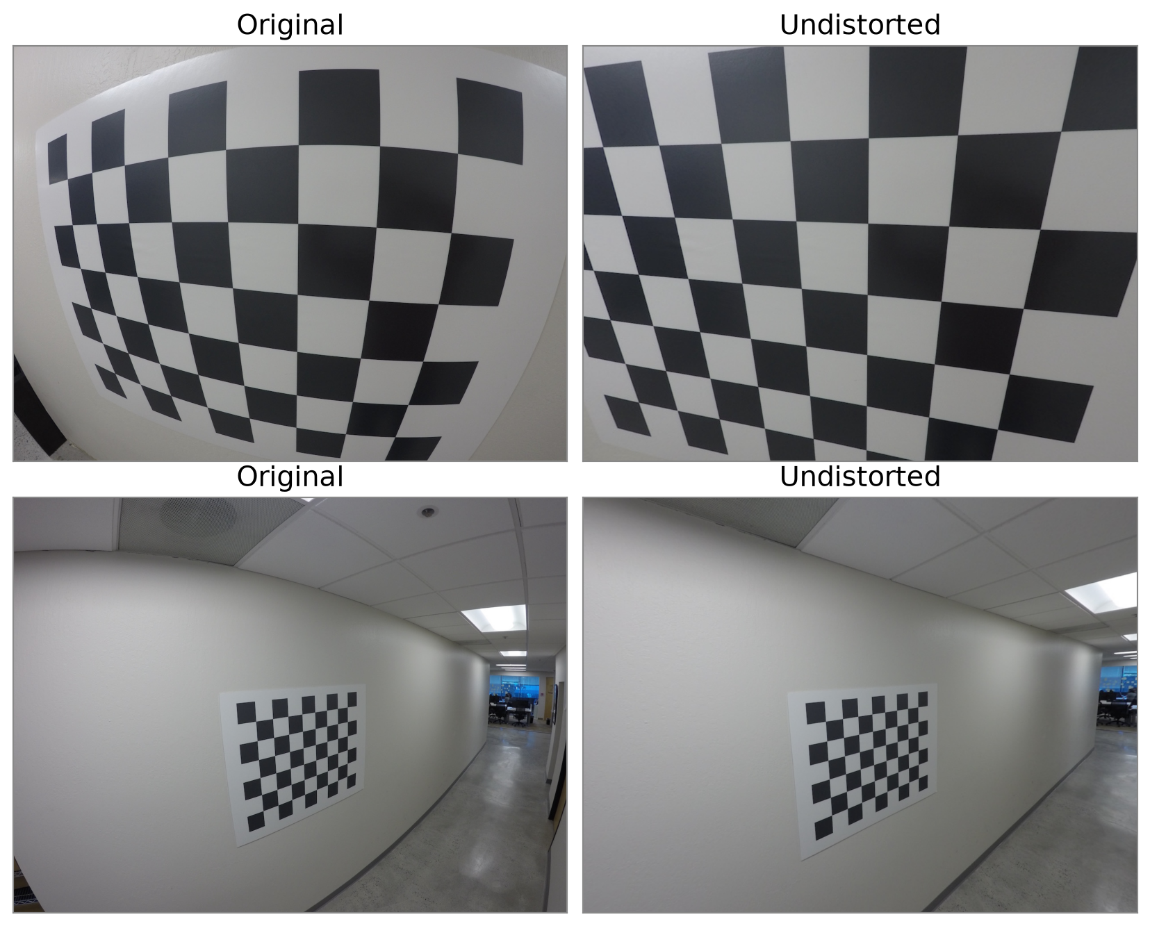
  • After \(\mathbf{K}\) and \(\mathbf{d}\) are found, they can be used to map every pixel back to where a pinhole camera would have seen it:
undistorted = cv2.undistort(img, K, dist)
  • Straight lines in the scene become straight in the image.
  • This can crop the image: the stretched corners fall outside the frame.
Full Calibration Code

from pathlib import Path

import cv2
import numpy as np

# Calibration images and the checkerboard geometry.
calib_files = sorted(Path("assets/12_camera_calibration/calibration").glob("*.jpg"))
pattern = (8, 6)   # inner corners per row, per column
square = 80.0      # square size in mm

# 3D corners in the board frame b: (X, Y, 0), in the same order as the detected corners.
objp = np.zeros((pattern[0] * pattern[1], 3), np.float32)
objp[:, :2] = np.mgrid[0:pattern[0], 0:pattern[1]].T.reshape(-1, 2) * square

criteria = (cv2.TERM_CRITERIA_EPS + cv2.TERM_CRITERIA_MAX_ITER, 30, 1e-3)

# Steps 1-2: detect the corners in every image and match them to the board points.
obj_points, img_points = [], []
for path in calib_files:
    gray = cv2.imread(str(path), cv2.IMREAD_GRAYSCALE)
    found, corners = cv2.findChessboardCorners(gray, pattern)
    if not found:
        print(f"Board not found in {path.name}, skipping")
        continue
    corners = cv2.cornerSubPix(gray, corners, (11, 11), (-1, -1), criteria)
    obj_points.append(objp)
    img_points.append(corners)

image_size = gray.shape[::-1]   # (width, height)

# Step 3: calibrate.
rms, K, dist, rvecs, tvecs = cv2.calibrateCamera(
    obj_points, img_points, image_size, None, None)

print(f"Views used: {len(obj_points)} of {len(calib_files)}")
print(f"RMS reprojection error: {rms:.3f} px")
print("K =\n", K)
print("dist (k1, k2, p1, p2, k3) =", dist.ravel())

# Undistort an image with the calibrated K and dist.
img = cv2.imread(str(calib_files[0]))
undistorted = cv2.undistort(img, K, dist)
cv2.imwrite("undistorted.jpg", undistorted)

Collecting Useful Calibration Images

  • Fix the camera settings first: focus, zoom, and resolution. Changing them changes \(\mathbf{K}\).
  • Use a flat, rigid board, and measure its square size.
  • Take 20–30 sharp images: no motion blur, even lighting, no glare.
  • Vary the orientation: tilt the board up to about \(45^\circ\) in different directions.
  • Cover the whole image, especially the corners, where distortion is largest.
  • Vary the distance, but keep the board large enough for accurate corners.
  • Check that each image is detected, and look at the result before collecting more.
Checking the Results: Error per View
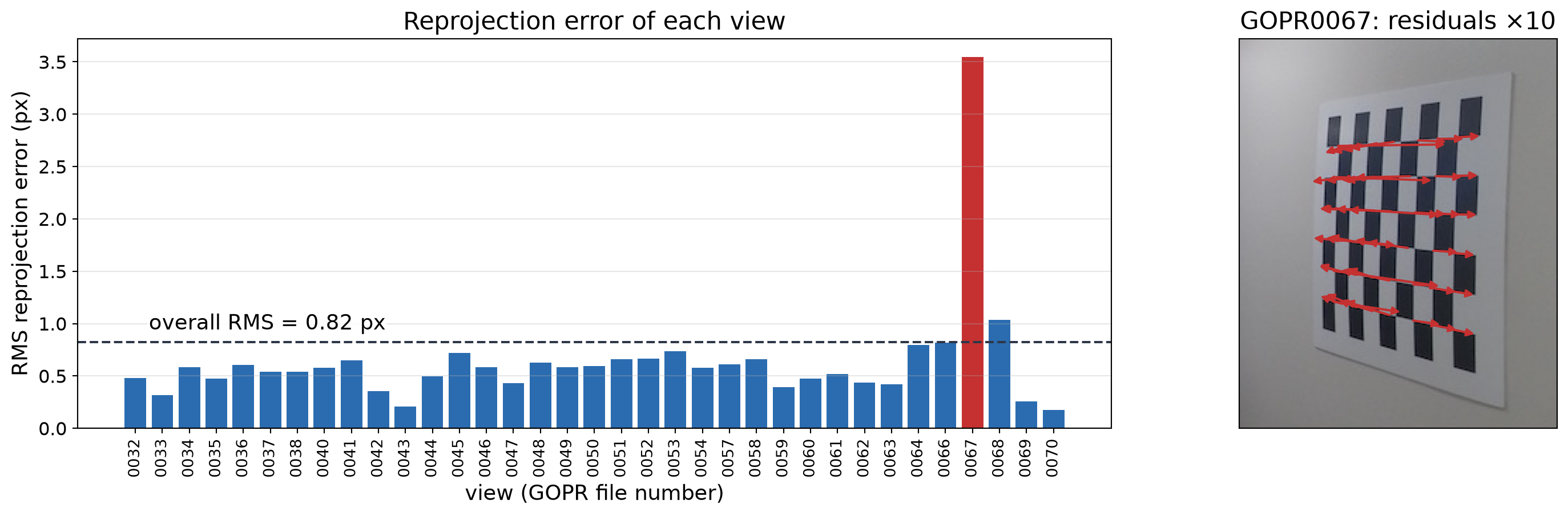
  • It’s good to check the per-view reprojection errors, not just the overall calibration RMS.
  • In our example, most views have an error below \(1\) px, but one has \(3.5\) px: about \(6\)x the median.
  • That is due to a board that is far away, so its corners are poorly localized.
  • One bad view can impact the calibration accuracy, so it is worth removing it and recalibrating.

Remove Outliers and Recalibrate

keep = [j for j in range(len(img_points)) if per_view[j] < 2.0]
(rms2, K2, dist2, rvecs2, tvecs2,
 std_intrinsics, std_extrinsics, per_view_errors) = cv2.calibrateCameraExtended(
    [obj_points[j] for j in keep], [img_points[j] for j in keep], image_size, None, None)
  • Dropping one bad view lowers the RMS error from 0.82 to 0.57 px.
  • The \(\pm\) values are one standard deviation, from std_intrinsics: all well below one pixel.
  • Remove views only for a reason (blur, tiny board, wrong detection), not just to lower the number.
All views Outlier removed
Views 35 34
RMS reprojection error (px) 0.82 0.57
\(f_x\) (px) 560.0 \(\pm\) 1.0 560.4 \(\pm\) 0.7
\(f_y\) (px) 561.1 \(\pm\) 0.9 561.4 \(\pm\) 0.6
\(c_x\) (px) 651.1 \(\pm\) 0.3 651.1 \(\pm\) 0.2
\(c_y\) (px) 498.9 \(\pm\) 0.5 499.0 \(\pm\) 0.3
\(k_1\) -0.2326 \(\pm\) 0.0009 -0.2328 \(\pm\) 0.0006
\(k_2\) 0.0615 \(\pm\) 0.0006 0.0616 \(\pm\) 0.0004

Key Takeaways

  • Geometric calibration estimates the intrinsic matrix \(\mathbf{K}\), the lens distortion \(\mathbf{d}\), and the pose of the target in each view.
  • With a known 3D target, the camera matrix \(\mathbf{P}\) follows linearly (DLT), and \(\mathbf{K}\), \({}^{c}\mathbf{R}_{w}\), \({}^{c}\mathbf{t}_{w}\) follow from it. In practice this is only an initial guess.
  • Calibration minimizes the reprojection error (in pixels) over all parameters, including distortion, with nonlinear least squares.
  • In OpenCV: findChessboardCorners → cornerSubPix → calibrateCamera → undistort.
  • Use 20–30 sharp views, tilted in different directions, that cover the whole image, especially its corners.
  • Check the per-view errors, not just the overall RMS; remove bad views for a reason and recalibrate.
  • Very wide lenses may need the fisheye (or omnidirectional) model.