Lecture 13 — Two-View Geometry

Lecture 13

Kaveh Fathian

Computer Science Department, Colorado School of Mines

Learning Objectives

By the end of this lecture, you should be able to:

  • Describe epipolar geometry, and use the fundamental and essential matrices to map a pixel in one image to its epipolar line in the other.
  • Estimate \(\mathbf{F}\) and \(\mathbf{E}\) from feature matches with OpenCV, using RANSAC to reject wrong matches.
  • Tell when a homography relates two views instead (planar scene, pure rotation, distant scene), and estimate one.
  • Recover the relative camera pose, triangulate matched points into a 3D point cloud, and explain the limits of two-view reconstruction.

One View Loses Depth, Two Views Recover It

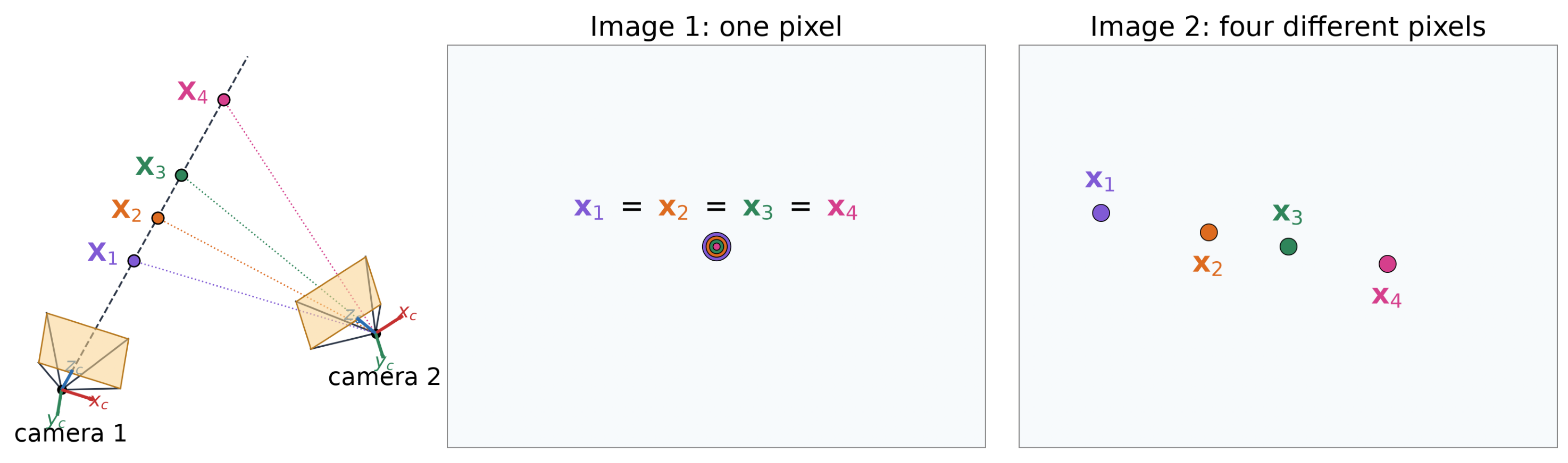
  • Every point on the ray from camera 1 lands on the same pixel \(\mathbf{x}_1\): Even when the camera matrix is known, one image cannot tell the depth \(\lambda_1\).
  • A second camera sees the same candidates at different pixels. Finding the match for \(\mathbf{x}_1\) determines its 3D point position.

The Two-View Problem

\[\lambda\,\mathbf{x} = \mathbf{K}\,\big[\,{}^{c}\mathbf{R}_{w} \mid {}^{c}\mathbf{t}_{w}\,\big]\;{}^{w}\mathbf{X}\]

Problem Pixels \(\mathbf{x}\) Intrinsics \(\mathbf{K}\) Extrinsics \({}^{c}\mathbf{R}_{w},\ {}^{c}\mathbf{t}_{w}\) 3D points \({}^{w}\mathbf{X}\)
Projection (simulate a camera) unknown known known known
Camera calibration known unknown unknown known
Two-view geometry known known unknown unknown
Triangulation known known known unknown
  • Calibration knows the 3D points and solves for intrinsics and extrinsics. In two-view geometry, 3D points and extrinsics are unknown.
  • Two-view geometry recovers the relative pose between two cameras. We assume one camera has the world frame, so its extrinsics are trivial. The second camera’s extrinsics are unknown, as is the 3D point: \[ \underbrace{\lambda_1\vphantom{\big[{}^{2}\mathbf{R}_{1}\big]}}_{\color{#c53030}{\text{unknown}}}\; \underbrace{\mathbf{x}_1\vphantom{\big[{}^{2}\mathbf{R}_{1}\big]}}_{\color{#2f855a}{\text{known}}} = \underbrace{\mathbf{K}\vphantom{\big[{}^{2}\mathbf{R}_{1}\big]}}_{\color{#2f855a}{\text{known}}}\; \underbrace{\big[\,\mathbf{I} \mid \mathbf{0}\,\big]}_{\color{#2f855a}{\text{known}}}\; \underbrace{{}^{1}\mathbf{X}\vphantom{\big[{}^{2}\mathbf{R}_{1}\big]}}_{\color{#c53030}{\text{unknown}}} \qquad\qquad \underbrace{\lambda_2\vphantom{\big[{}^{2}\mathbf{R}_{1}\big]}}_{\color{#c53030}{\text{unknown}}}\; \underbrace{\mathbf{x}_2\vphantom{\big[{}^{2}\mathbf{R}_{1}\big]}}_{\color{#2f855a}{\text{known}}} = \underbrace{\mathbf{K}\vphantom{\big[{}^{2}\mathbf{R}_{1}\big]}}_{\color{#2f855a}{\text{known}}}\; \underbrace{\big[\,{}^{2}\mathbf{R}_{1} \mid {}^{2}\mathbf{t}_{1}\,\big]}_{\color{#c53030}{\text{unknown}}}\; \underbrace{{}^{1}\mathbf{X}\vphantom{\big[{}^{2}\mathbf{R}_{1}\big]}}_{\color{#c53030}{\text{unknown}}} \]

Epipolar Geometry

Term Definition
Baseline Line through the camera centers \({}^{w}\mathbf{C}_1\), \({}^{w}\mathbf{C}_2\)
Epipolar plane Plane through the baseline and \({}^{w}\mathbf{X}\)
Epipolar lines \({}^{1}\ell\), \({}^{2}\ell\) Where the epipolar plane cuts each image plane
Epipoles \({}^{1}\mathbf{e}\), \({}^{2}\mathbf{e}\) Where the baseline cuts each image plane
  • The pixels \({}^{1}\mathbf{x}\) and \({}^{2}\mathbf{x}\) lie on \({}^{1}\ell\) and \({}^{2}\ell\).
  • Each epipole is the image of the other camera’s center.
3D view with orbit slider
view: top behind cameras

The Epipolar Constraint

3D view with orbit slider
view: top behind cameras
  • Epipolar constraint: the match \({}^{2}\mathbf{x}\) of \({}^{1}\mathbf{x}\) must lie on the epipolar line \({}^{2}\ell\), whatever the depth of \({}^{w}\mathbf{X}\).
  • Matching becomes a 1D search along a line instead of a 2D search over the whole image.

All Epipolar Lines Meet at the Epipole

3D view with orbit slider
view: top behind cameras
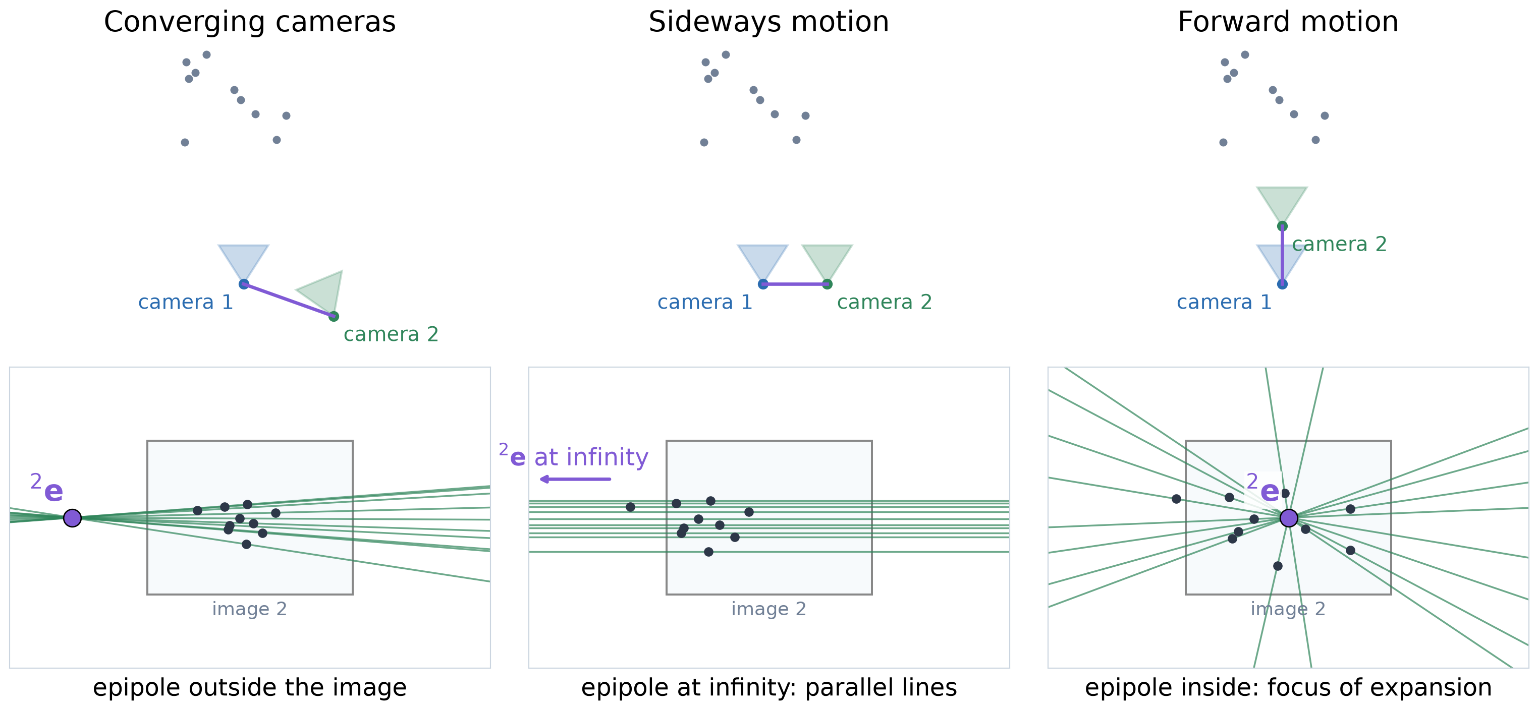
  • Every epipolar plane contains the baseline, so every epipolar line in an image passes through that image’s epipole.
  • The lines come in corresponding pairs: one plane gives one line in each image. Here both epipoles lie outside the images.

Where Is the Epipole?
Lines in Homogeneous Coordinates
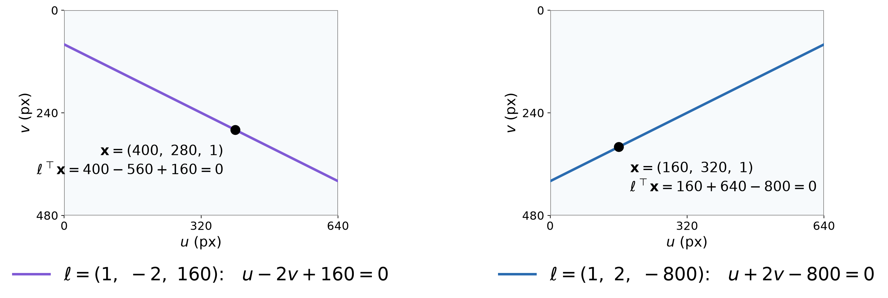
  • A line in the image can be modelled as the set of pixels \((u, v)\) that satisfy \(a\,u + b\,v + c = 0\).
  • Using homogeneous coordinates \(\mathbf{x} = (u, v, 1)^{\top}\), and representing the lines coefficients as \(\ell = (a, b, c)^{\top}\): \[ \mathbf{x} \text{ is on line } \ell \quad\Longleftrightarrow\quad \ell^{\top}\mathbf{x} = a\,u + b\,v + c = 0 \]

The Fundamental Matrix
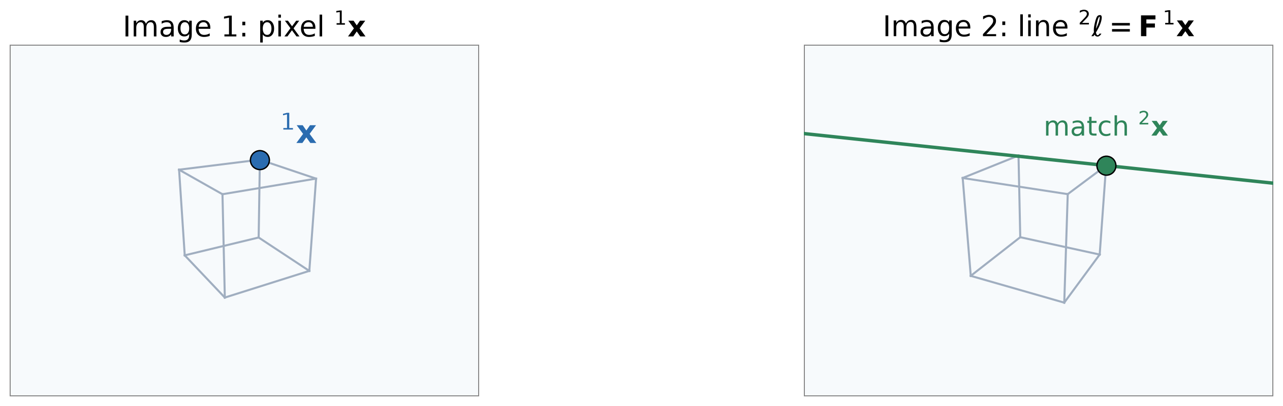
  • The fundamental matrix \(\mathbf{F}\) is a \(3\times3\) matrix that maps a pixel in image 1 to its epipolar line in image 2:

\[ \mathbf{F}\,{}^{1}\mathbf{x} = \underbrace{{}^{2}\ell}_{(a,\,b,\,c)^{\top}} \qquad\Longrightarrow\qquad \bbox[border: 2px solid #c53030; padding: 2px 6px]{\underbrace{{}^{2}\mathbf{x}^{\top}\,\mathbf{F}\,{}^{1}\mathbf{x} = 0}_{a\,u_2\,+\,b\,v_2\,+\,c\,=\,0}} \;\;{\color{#c53030}{\begin{array}{l}\textbf{fundamental matrix}\\ \textbf{constraint}\end{array}}} \]

  • The same \(\mathbf{F}\) works for every image point.
  • In the other direction, \({}^{1}\ell = \mathbf{F}^{\top}\,{}^{2}\mathbf{x}\).

The Fundamental Matrix: A Numerical Example

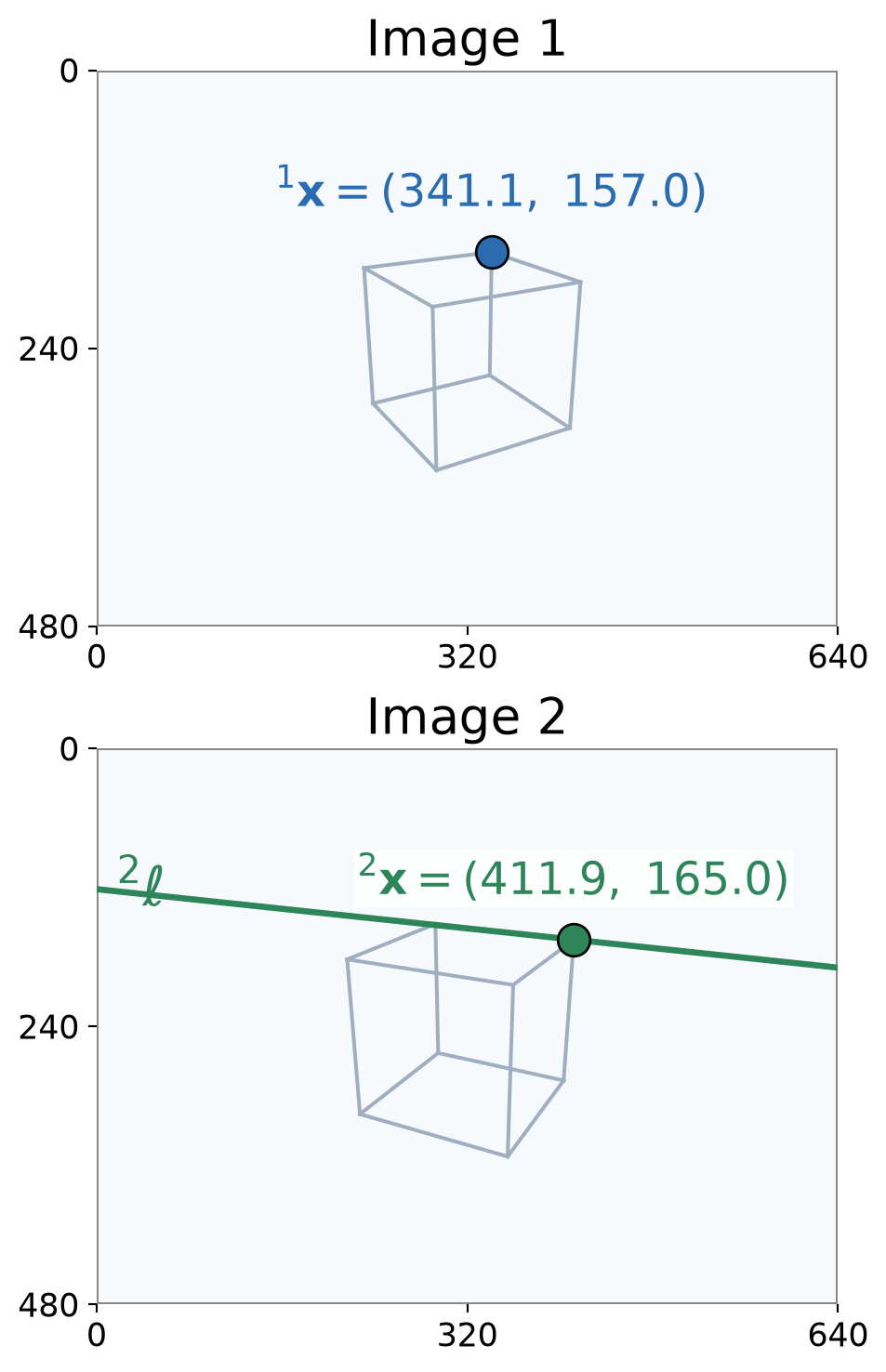
\[{}^{1}\mathbf{x} = (341.1,\ 157.0,\ 1)^{\top},\qquad{}^{2}\mathbf{x} = (411.9,\ 165.0,\ 1)^{\top}\]

\[\mathbf{F} = \begin{bmatrix} 0 & 1.26{\times}10^{-4} & -5.64{\times}10^{-3} \\ 1.57{\times}10^{-4} & -1.31{\times}10^{-5} & -0.19 \\ -4.91{\times}10^{-3} & 0.11 & 1.00 \end{bmatrix}\]

\[\begin{aligned} {}^{2}\ell &= \mathbf{F}\,{}^{1}\mathbf{x} = (0.105,\ -0.994,\ 120.7)^{\top} \\ \text{line }{}^{2}\ell &:\ \ 0.105\,u -0.994\,v +120.7 = 0 \end{aligned}\]

\[\begin{aligned} {}^{2}\mathbf{x}^{\top}\mathbf{F}\,{}^{1}\mathbf{x} = {}^{2}\mathbf{x}^{\top}\,{}^{2}\ell &= 0.105\cdot411.9 -0.994\cdot165.0 +120.7 \\ &= 0.00 \end{aligned}\]
(Supplementary) Deriving the Fundamental Matrix

  • Pixel \({}^{i}\mathbf{x}\)’s viewing ray has direction \(\mathbf{K}^{-1}\,{}^{i}\mathbf{x}\) in camera \(i\)’s frame.
  • In camera 2’s frame, three vectors lie in the epipolar plane:
    • \(\mathbf{K}^{-1}\,{}^{2}\mathbf{x}\): camera 2’s ray
    • \({}^{2}\mathbf{t}_{1}\): the baseline (to camera 1)
    • \({}^{2}\mathbf{R}_{1}\,\mathbf{K}^{-1}\,{}^{1}\mathbf{x}\): camera 1’s ray, in frame 2
  • So the first is perpendicular to the normal \(\mathbf{n}\) of the other two:

\[ \big({\color{#2f855a}{\mathbf{K}^{-1}\,{}^{2}\mathbf{x}}}\big)^{\top} \underbrace{\big({\color{#805ad5}{{}^{2}\mathbf{t}_{1}}} \times {\color{#2b6cb0}{{}^{2}\mathbf{R}_{1}\,\mathbf{K}^{-1}\,{}^{1}\mathbf{x}}}\big)}_{\mathbf{n}} = 0 \] \[ \Longrightarrow\quad {}^{2}\mathbf{x}^{\top}\, \underbrace{\mathbf{K}^{-\top}\,[{}^{2}\mathbf{t}_{1}]_{\times}\,{}^{2}\mathbf{R}_{1}\,\mathbf{K}^{-1}}_{\mathbf{F}}\; {}^{1}\mathbf{x} = 0 \]

3D view with orbit slider
view: top behind cameras
\([\mathbf{t}]_{\times}\) writes the cross product with \(\mathbf{t} = (t_x, t_y, t_z)^{\top}\) as a matrix:

\[ \mathbf{t}\times\mathbf{v} = [\mathbf{t}]_{\times}\,\mathbf{v}, \qquad [\mathbf{t}]_{\times} = \begin{bmatrix} 0 & -t_z & t_y \\ t_z & 0 & -t_x \\ -t_y & t_x & 0 \end{bmatrix} \]

The Essential Matrix

  • The fundamental matrix \(\mathbf{F}\) is the epipolar constraint for uncalibrated cameras, in pixel coordinates: \[ {}^{2}\mathbf{x}^{\top}\, \underbrace{\mathbf{K}^{-\top}\,[{}^{2}\mathbf{t}_{1}]_{\times}\,{}^{2}\mathbf{R}_{1}\,\mathbf{K}^{-1}}_{\mathbf{F}}\; {}^{1}\mathbf{x} = 0 \]

  • The middle part of \(\mathbf{F}\) is the essential matrix: \[\mathbf{E} = [{}^{2}\mathbf{t}_{1}]_{\times}\,{}^{2}\mathbf{R}_{1}\]

  • It is the epipolar constraint for calibrated cameras, in normalized coordinates \(\hat{\mathbf{x}} = \mathbf{K}^{-1}\mathbf{x}\) (ray directions): \[ \bbox[border: 2px solid #c53030; padding: 2px 6px]{{}^{2}\hat{\mathbf{x}}^{\top}\,\mathbf{E}\,{}^{1}\hat{\mathbf{x}} = 0} \;\;{\color{#c53030}{\begin{array}{l}\textbf{essential matrix}\\ \textbf{constraint}\end{array}}} \]

  • It contains only the relative pose of the two cameras, nothing about the scene or the intrinsics.

For the same point as before:

\[\mathbf{K} = \begin{bmatrix} 500 & 0 & 320 \\ 0 & 500 & 240 \\ 0 & 0 & 1 \end{bmatrix}\]

\[\begin{aligned} {}^{1}\mathbf{x} &= (341.1,\ 157.0,\ 1)^{\top} \\ {}^{2}\mathbf{x} &= (411.9,\ 165.0,\ 1)^{\top} \\[4pt] {}^{1}\hat{\mathbf{x}} &= \mathbf{K}^{-1}\,{}^{1}\mathbf{x} = (0.042,\ -0.166,\ 1)^{\top} \\ {}^{2}\hat{\mathbf{x}} &= \mathbf{K}^{-1}\,{}^{2}\mathbf{x} = (0.184,\ -0.150,\ 1)^{\top} \end{aligned}\]

\[\mathbf{E} = \begin{bmatrix} 0 & -1.29 & -0.5 \\ -1.61 & 0.13 & 2.83 \\ -0.67 & -2.97 & 0 \end{bmatrix}\]

\[{}^{2}\hat{\mathbf{x}}^{\top}\mathbf{E}\,{}^{1}\hat{\mathbf{x}} = 0.00\]

Estimating F With OpenCV

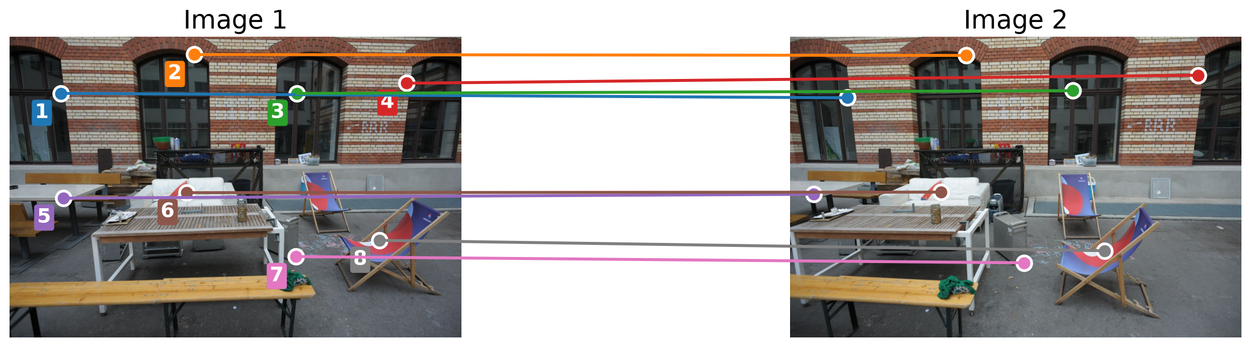
  1. Detect and match feature points in both images.
  2. Collect the matched pixels: pts1, pts2, \(N\times2\) arrays in the same order.
  3. Estimate \(\mathbf{F}\) (or \(\mathbf{E}\)) from these correspondences.
# Uncalibrated: 
F, _ = cv2.findFundamentalMat(pts1, pts2,
                              cv2.FM_8POINT)
# Calibrated: 
E, _ = cv2.findEssentialMat(pts1, pts2, K)

Results on these images (K from the dataset):

\[\mathbf{F} = \begin{bmatrix} 4.01{\times}10^{-8} & 5.08{\times}10^{-6} & -1.69{\times}10^{-3} \\ 1.13{\times}10^{-7} & 5.48{\times}10^{-6} & -0.03 \\ 1.46{\times}10^{-4} & 0.02 & 1.00 \end{bmatrix}\]

\[\mathbf{E} = \begin{bmatrix} -8.05{\times}10^{-4} & -0.02 & 3.15{\times}10^{-3} \\ 0.12 & -4.67{\times}10^{-4} & -0.70 \\ 0.01 & 0.71 & 1.70{\times}10^{-3} \end{bmatrix}\]

Estimating F and E With OpenCV: Full Code

import cv2
import numpy as np

# Two views of the same scene.
img1 = cv2.imread("assets/13_two_view_geometry/frame1.JPG", cv2.IMREAD_GRAYSCALE)
img2 = cv2.imread("assets/13_two_view_geometry/frame2.JPG", cv2.IMREAD_GRAYSCALE)

# Intrinsics of the camera
K = np.array([[3409.58,    0.0, 3115.16],
              [   0.0, 3409.44, 2064.73],
              [   0.0,    0.0,     1.0]])
K[:2] *= 0.2

# 1. Detect and match features: SIFT with Lowe's ratio test.
sift = cv2.SIFT_create()
kp1, des1 = sift.detectAndCompute(img1, None)
kp2, des2 = sift.detectAndCompute(img2, None)
knn = cv2.BFMatcher(cv2.NORM_L2).knnMatch(des1, des2, k=2)
good = [m for m, n in knn if m.distance < 0.75 * n.distance]

# 2. Matched pixels, N x 2, in the same order.
pts1 = np.float32([kp1[m.queryIdx].pt for m in good])
pts2 = np.float32([kp2[m.trainIdx].pt for m in good])

# 3. Estimate F (uncalibrated) and E (calibrated).
F, _ = cv2.findFundamentalMat(pts1, pts2, cv2.FM_8POINT)
E, _ = cv2.findEssentialMat(pts1, pts2, K)

print(f"{len(good)} matches")
print("F =\n", F / F[2, 2])
print("E =\n", E)

(Supplementary) The Eight-Point Algorithm

  • OpenCV’s cv2.findFundamentalMat(..., cv2.FM_8POINT) implements the eight-point algorithm to estimate the fundamental matrix (Hartley & Zisserman, 2004, §11.1.1). The steps are:

  • One row per match. With \({}^{1}\mathbf{x} = (u_1, v_1, 1)^{\top}\), \({}^{2}\mathbf{x} = (u_2, v_2, 1)^{\top}\) and \(\mathbf{f} = (F_{11}, F_{12}, \dots, F_{33})^{\top}\), the constraint \({}^{2}\mathbf{x}^{\top}\mathbf{F}\,{}^{1}\mathbf{x} = 0\) is linear in \(\mathbf{f}\): \[ \big[\,u_2u_1,\ u_2v_1,\ u_2,\ v_2u_1,\ v_2v_1,\ v_2,\ u_1,\ v_1,\ 1\,\big]\;\mathbf{f} = 0 \]

  • Solve. Stack \(N \ge 8\) rows into \(\mathbf{A}\) (\(N\times 9\)). \(\mathbf{f}\) is the right singular vector of \(\mathbf{A}\) with the smallest singular value, as in the DLT of Lecture 12.

  • Force rank 2. A true \(\mathbf{F}\) has \(\det\mathbf{F} = 0\): that is what makes all epipolar lines meet at the epipole. With noise, the solution has rank 3. With \(\mathbf{F} = \mathbf{U}\,\mathrm{diag}(\sigma_1, \sigma_2, \sigma_3)\,\mathbf{V}^{\top}\), set \(\sigma_3 = 0\): the closest rank-2 matrix.

  • Normalize first. Pixel values make the entries of \(\mathbf{A}\) range from 1 to \(\sim\!10^{5}\), which makes the solution sensitive to noise. Shift each image’s points to zero mean and scale them to mean distance \(\sqrt{2}\) (transforms \(\mathbf{T}_1\), \(\mathbf{T}_2\)), solve, then undo: \(\mathbf{F} = \mathbf{T}_2^{\top}\,\tilde{\mathbf{F}}\,\mathbf{T}_1\).

How Many Matches Do We Need?

Algorithm Estimates Needs \(\mathbf{K}\)? Matches Solutions OpenCV
Eight-point \(\mathbf{F}\) No 8 or more 1 findFundamentalMat(..., cv2.FM_8POINT)
Seven-point \(\mathbf{F}\) No exactly 7 1 or 3 findFundamentalMat(..., cv2.FM_7POINT)
Five-point \(\mathbf{E}\) Yes 5 or more up to 10 findEssentialMat(..., K)
  • Each algorithm needs a minimum number of matches or correspondences \({}^{1}\mathbf{x}_j \leftrightarrow {}^{2}\mathbf{x}_j\) to estimate \(\mathbf{F}\) or \(\mathbf{E}\).
  • The seven- and five-point algorithms can return several solutions; the other correspondences are used to pick the one most of them agree with.
  • Why use as few matches as possible?

Not All Matches Are Correct
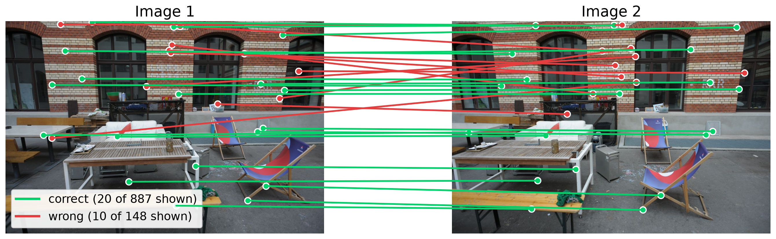
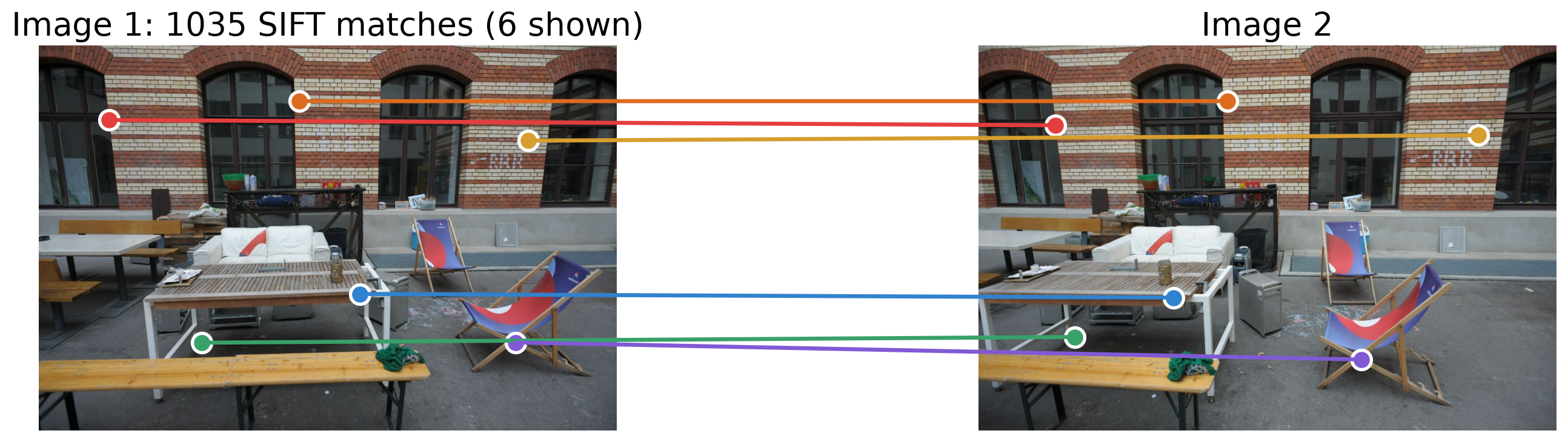
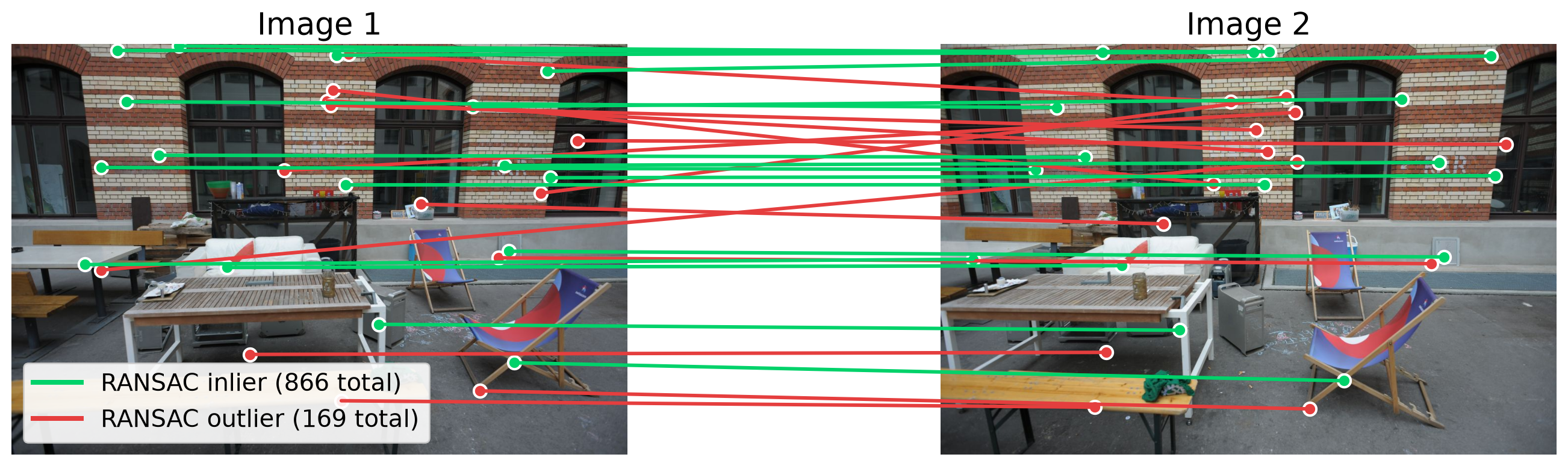
  • Of the 1035 SIFT matches, 148 are wrong: they do not fit the scene’s true epipolar geometry.

  • Why use as few matches as possible? In practice, some matches are wrong

  • Every match used in an algorithm must be correct to estimate \(\mathbf{F}\) or \(\mathbf{E}\) correctly.

  • The more matches we use, the more likely it is that at least one of them is wrong.

  • How can we robustly estimate \(\mathbf{F}\) or \(\mathbf{E}\) from a set of matches that contains some wrong ones?

RANSAC: Fitting a Line With Outliers

  • RANdom SAmple Consensus (RANSAC): the model that most points agree with wins.

RANSAC Algorithm

  1. Sample the minimum number of points needed to fit the model (2 for a line), at random.
  2. Fit the model to the sample.
  3. Score: count the inliers, the points within a threshold \(\tau\) of the model.
  4. Repeat 1–3 and keep the model with the most inliers.
  • Least squares uses every point, so outliers pull it away.
Calibration animation

Fitting a line with RANSAC.

Example: Estimating a Translation
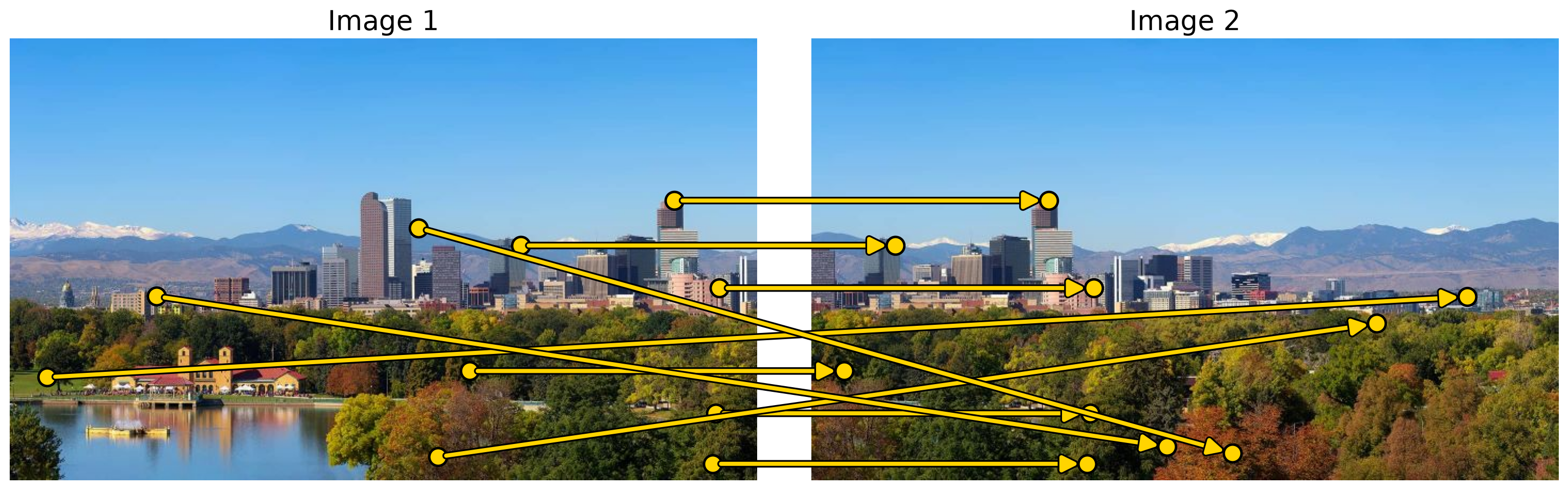
  • Image 2 is a sideways shift of image 1: the model is a translation, \({}^{2}\mathbf{x} = {}^{1}\mathbf{x} + \mathbf{t}\). Each match gives its own estimate \(\mathbf{t}_j = {}^{2}\mathbf{x}_j - {}^{1}\mathbf{x}_j\).

  • Correct matches all agree: their arrows are parallel and equally long. Wrong matches point anywhere.

  • Least squares averages all \(\mathbf{t}_j\), so the wrong matches pull it away: \(\mathbf{t}_{\text{LS}} = (-148,\ 15)\) px instead of \(\mathbf{t} = (-400,\ 0)\) px.

RANSAC for the Translation

Calibration animation
  • A translation needs one match: pick one at random (cyan), set \(\mathbf{t} = {}^{2}\mathbf{x}_j - {}^{1}\mathbf{x}_j\), and count the matches with \(\lVert {}^{2}\mathbf{x}_k - {}^{1}\mathbf{x}_k - \mathbf{t} \rVert < \tau\) (green).
  • The answer is the largest group of matches that agree, here the parallel arrows. Wrong matches rarely agree with each other.

RANSAC for F and E

RANSAC for F (or E)

  1. Sample 8 matches at random (7 for \(\mathbf{F}\) with the seven-point algorithm, 5 for \(\mathbf{E}\)).
  2. Estimate \(\mathbf{F}\) (or \(\mathbf{E}\)) from the sample.
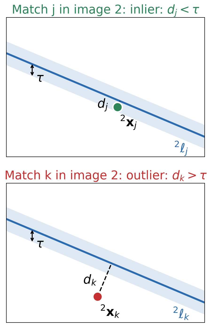
  3. Score: for every match, compute the distance \(d_j\) from \({}^{2}\mathbf{x}_j\) to its epipolar line \({}^{2}\ell_j = \mathbf{F}\,{}^{1}\mathbf{x}_j\). The match is an inlier if \(d_j < \tau\).
  4. Repeat 1–3 and keep the \(\mathbf{F}\) with the most inliers.
  5. Re-estimate \(\mathbf{F}\) from all of its inliers.
  • With \({}^{2}\ell_j = (a_j, b_j, c_j)^{\top}\), the distance in pixels is \[ d_j = \frac{\big|\,{}^{2}\mathbf{x}_j^{\top}\,\mathbf{F}\,{}^{1}\mathbf{x}_j\big|}{\sqrt{a_j^2 + b_j^2}} \]
  • For \(\mathbf{E}\), measure in pixels with \(\mathbf{F} = \mathbf{K}^{-\top}\mathbf{E}\,\mathbf{K}^{-1}\). A typical \(\tau\) is 1 px.
(Supplementary) How Many RANSAC Trials?

  • One trial succeeds if all \(s\) sampled matches are inliers. With outlier ratio \(\varepsilon\), this has probability \((1-\varepsilon)^{s}\).
  • All \(N\) trials fail with probability \(\big(1-(1-\varepsilon)^{s}\big)^{N}\). To succeed with probability \(p\), set this to \(1 - p\): \[ N = \frac{\log(1-p)}{\log\!\big(1-(1-\varepsilon)^{s}\big)} \]
  • \(\varepsilon\) is unknown in advance. RANSAC starts with a pessimistic guess and lowers \(N\) each time it finds a model with more inliers.

Trials \(N\) needed for \(p = 0.99\):

Model \(s\) 10% 20% 30% 40% 50%
Translation 1 2 3 4 6 7
Line 2 3 5 7 11 17
\(\mathbf{E}\), 5-point 5 6 12 26 57 146
\(\mathbf{F}\), 7-point 7 8 20 54 163 588
\(\mathbf{F}\), 8-point 8 9 26 78 272 1,177

Columns: outlier ratio \(\varepsilon\).

  • Fewer matches per sample, far fewer trials: this is why we use the minimum number of matches.
  • For the frame1/frame2 matches, \(\varepsilon \approx 14\%\), so the eight-point algorithm needs only 14 trials.

RANSAC With OpenCV

F, mask = cv2.findFundamentalMat(pts1, pts2,
                    cv2.FM_RANSAC, 1.0, 0.999)
E, mask = cv2.findEssentialMat(pts1, pts2, K,
                    cv2.RANSAC, 0.999, 1.0)
inliers1 = pts1[mask.ravel() == 1]
  • 1.0: threshold \(\tau\) in pixels. 0.999: probability \(p\) of sampling at least one all-inlier set.
  • mask is 1 for the inliers. findEssentialMat uses RANSAC by default.

Compared with the ground truth:

Method Matches used Median error
Eight-point, all matches 1035 7.56 px
RANSAC, \(\mathbf{F}\) 866 (851 correct) 0.24 px
RANSAC, \(\mathbf{E}\) 870 (869 correct) 0.08 px

Median error: distance of the correct matches to their estimated epipolar lines.

The Homography Matrix
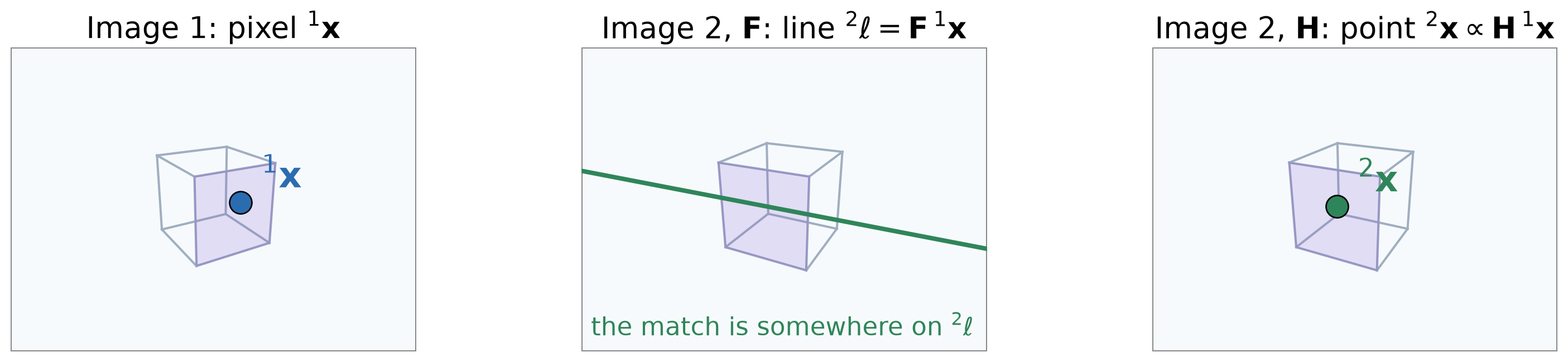
  • For points on one plane (cube’s front face), a \(3\times3\) homography \(\mathbf{H}\) maps \({}^{1}\mathbf{x}\) in image 1 to its match in \({}^{2}\mathbf{x}\) image 2: \[ \bbox[border: 2px solid #c53030; padding: 2px 6px]{\,{}^{2}\mathbf{x} = \mathbf{H}\,{}^{1}\mathbf{x}} \;\;{\color{#c53030}{\begin{array}{l}\textbf{homography constraint}\end{array}}} \]

In homogeneous coordinates; divide \(\mathbf{H}\,{}^{1}\mathbf{x}\) by its third entry.

Fundamental matrix \(\mathbf{F}\) Homography \(\mathbf{H}\)
Maps \({}^{1}\mathbf{x}\) to a line \({}^{2}\ell\) a point \({}^{2}\mathbf{x}\)
Holds for any scene one plane, or a rotating camera

The Homography: A Numerical Example

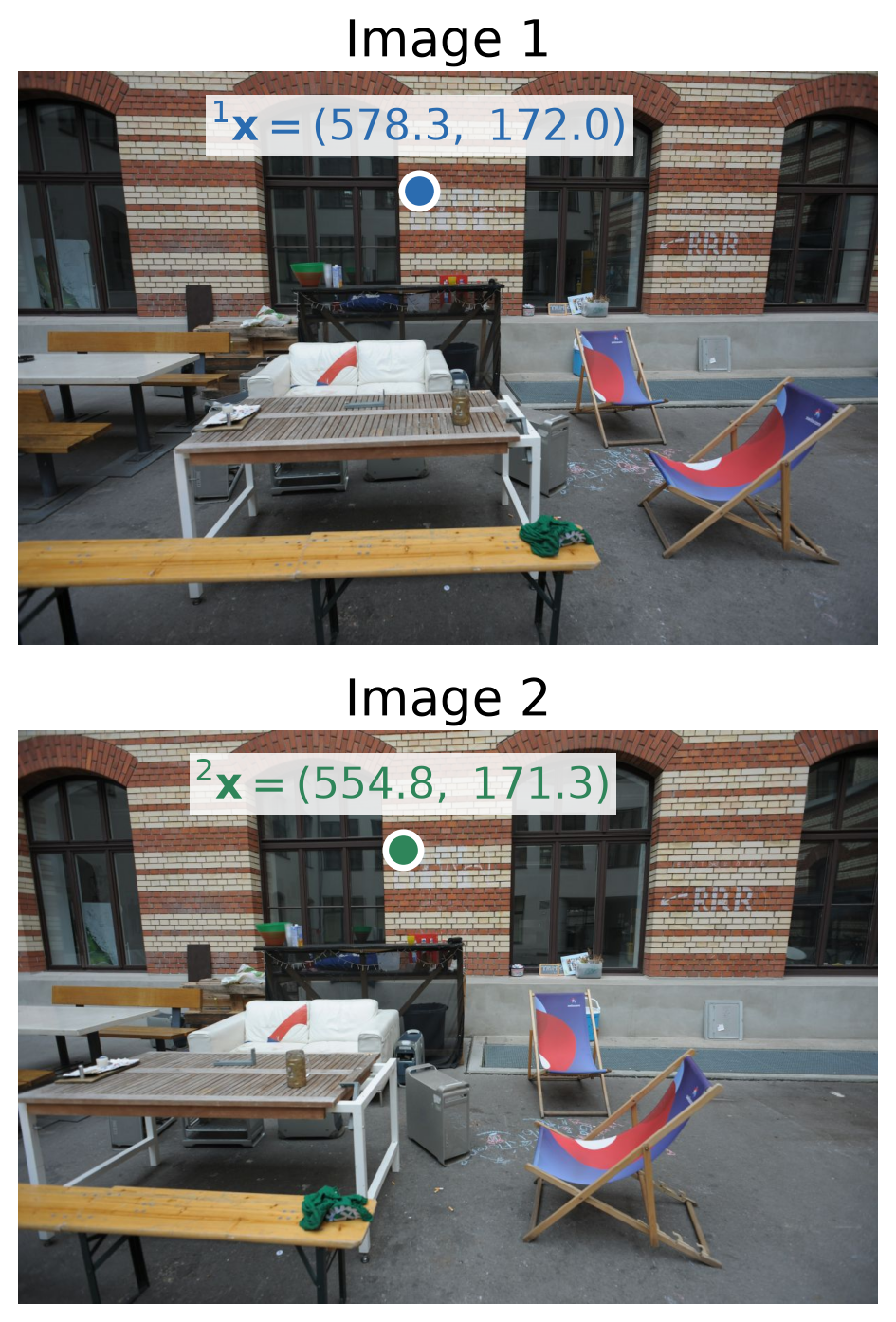
\[{}^{1}\mathbf{x} = (578.3,\ 172.0,\ 1)^{\top}\]

\[\mathbf{H} = \begin{bmatrix} 0.781 & 7.975{\times}10^{-3} & 42.418 \\ -0.057 & 0.898 & 31.333 \\ -1.865{\times}10^{-4} & 2.647{\times}10^{-6} & 1.000 \end{bmatrix}\]

  • \(\mathbf{H}\): the homography of the wall.

\[\begin{aligned} \mathbf{H}\,{}^{1}\mathbf{x} &= (495.2,\ 152.9,\ 0.893)^{\top} \\ {}^{2}\mathbf{x} &= \Big(\tfrac{495.2}{0.893},\ \tfrac{152.9}{0.893}\Big) = (554.8,\ 171.3) \end{aligned}\]
When Does One Homography Relate Two Views?
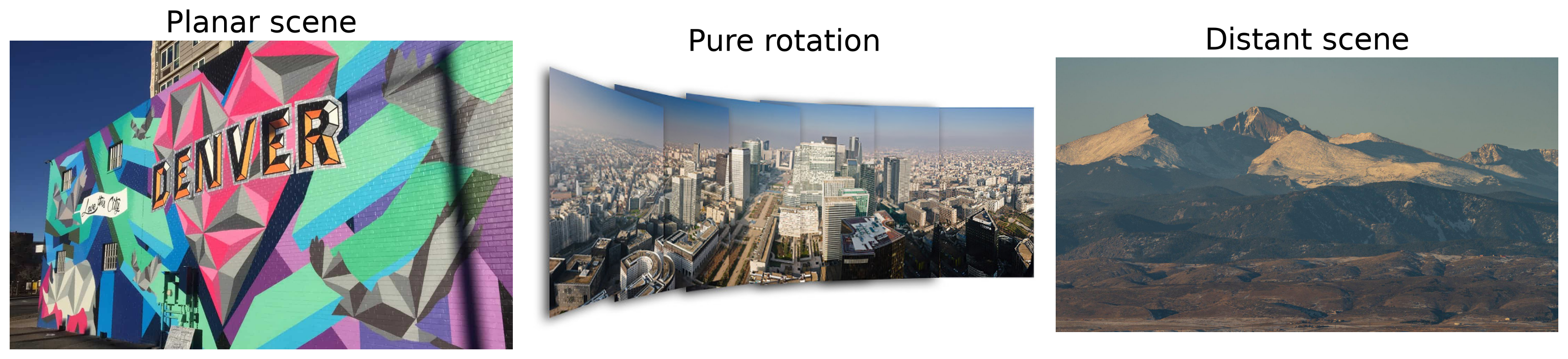
  • Planar scene: all points lie on one plane (e.g., a wall or floor).
  • Pure rotation: the camera turns about its center (e.g., when shooting a panorama).
  • Distant scene: objects are far away, so depth differences are tiny compared with the mean distance, making the scene nearly planar.
  • Otherwise:
    • In a 3D scene: points at different depths shift by different amounts. One \(\mathbf{H}\) cannot map them all; use \(\mathbf{F}\) or \(\mathbf{E}\).
    • When the 3D scene has multiple planar objects, each plane requires its own homography.

(Supplementary) Where Does the Homography Come From?

  • A plane, in camera 1’s frame: \(\mathbf{n}^{\top}\,{}^{1}\mathbf{X} = d\), with unit normal \(\mathbf{n}\) and distance \(d\) from camera 1. So \(\mathbf{n}^{\top}\,{}^{1}\mathbf{X}/d = 1\) for its points.
  • Move a plane point to camera 2’s frame, and multiply \({}^{2}\mathbf{t}_{1}\) by that 1: \[ {}^{2}\mathbf{X} = {}^{2}\mathbf{R}_{1}\,{}^{1}\mathbf{X} + {}^{2}\mathbf{t}_{1}\,\frac{\mathbf{n}^{\top}\,{}^{1}\mathbf{X}}{d} = \Big({}^{2}\mathbf{R}_{1} + \frac{1}{d}\,{}^{2}\mathbf{t}_{1}\,\mathbf{n}^{\top}\Big)\,{}^{1}\mathbf{X} \]
  • With \({}^{1}\mathbf{X} = \lambda_1\mathbf{K}^{-1}\,{}^{1}\mathbf{x}\) and \(\lambda_2\,{}^{2}\mathbf{x} = \mathbf{K}\,{}^{2}\mathbf{X}\): \[ \frac{\lambda_2}{\lambda_1}\,{}^{2}\mathbf{x} = \underbrace{\mathbf{K}\Big({}^{2}\mathbf{R}_{1} + \frac{1}{d}\,{}^{2}\mathbf{t}_{1}\,\mathbf{n}^{\top}\Big)\mathbf{K}^{-1}}_{\mathbf{H}}\;{}^{1}\mathbf{x} \]
3D view with orbit slider
view: top behind cameras
  • One \(\mathbf{H}\) for the whole image when:
    • Planar scene: every point satisfies \(\mathbf{n}^{\top}\,{}^{1}\mathbf{X} = d\).
    • Pure rotation: \({}^{2}\mathbf{t}_{1} = \mathbf{0}\), so \(\mathbf{H} = \mathbf{K}\,{}^{2}\mathbf{R}_{1}\mathbf{K}^{-1}\) for points at any depth.
    • Distant scene: \(d \gg \lVert{}^{2}\mathbf{t}_{1}\rVert\), so \(\mathbf{H} \approx \mathbf{K}\,{}^{2}\mathbf{R}_{1}\mathbf{K}^{-1}\).

(Supplementary) Estimating H: Direct Linear Transform

  • The basic solver for \(\mathbf{H}\) is the direct linear transform (DLT), the same as linear camera calibration. OpenCV’s cv2.findHomography uses DLT. The steps are:

  • Two rows per match. With \({}^{1}\mathbf{x} = (u_1, v_1, 1)^{\top}\), \({}^{2}\mathbf{x} = (u_2, v_2, 1)^{\top}\) and \(\mathbf{h}_i^{\top}\) the rows of \(\mathbf{H}\), the constraint gives \(u_2 = \frac{\mathbf{h}_1^{\top}\,{}^{1}\mathbf{x}}{\mathbf{h}_3^{\top}\,{}^{1}\mathbf{x}}\) and \(v_2 = \frac{\mathbf{h}_2^{\top}\,{}^{1}\mathbf{x}}{\mathbf{h}_3^{\top}\,{}^{1}\mathbf{x}}\). Multiplying out, both are linear in \(\mathbf{h} = (\mathbf{h}_1; \mathbf{h}_2; \mathbf{h}_3)\): \[ \begin{bmatrix} {}^{1}\mathbf{x}^{\top} & \mathbf{0}^{\top} & -u_2\,{}^{1}\mathbf{x}^{\top} \\ \mathbf{0}^{\top} & {}^{1}\mathbf{x}^{\top} & -v_2\,{}^{1}\mathbf{x}^{\top} \end{bmatrix} \mathbf{h} = \mathbf{0} \]

  • Solve. Stack \(N \ge 4\) matches into \(\mathbf{A}\) (\(2N\times 9\)). \(\mathbf{h}\) is the right singular vector of \(\mathbf{A}\) with the smallest singular value. Four matches (no three collinear) give exactly one \(\mathbf{H}\).

  • Normalize first, as in the eight-point algorithm: transform each image’s points to zero mean and mean distance \(\sqrt{2}\) (\(\mathbf{T}_1\), \(\mathbf{T}_2\)), solve, then undo: \(\mathbf{H} = \mathbf{T}_2^{-1}\,\tilde{\mathbf{H}}\,\mathbf{T}_1\).

Estimating H With OpenCV

H, mask = cv2.findHomography(pts1, pts2,
                             cv2.RANSAC, 2.0)
inliers1 = pts1[mask.ravel() == 1]
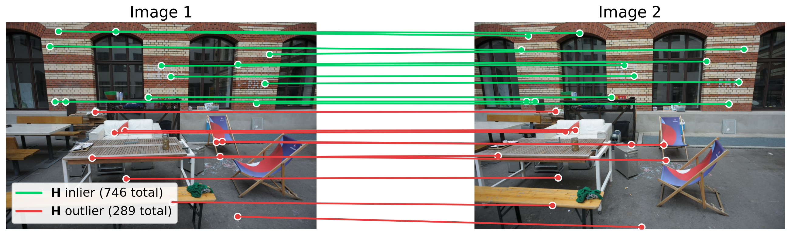
  • Same SIFT matches as for \(\mathbf{F}\). RANSAC samples 4 matches per trial, and finds the plane that most matches agree with: the wall.
  • 2.0: threshold \(\tau\) in pixels. mask is 1 for the inliers.
  • RANSAC error: the distance from \({}^{2}\mathbf{x}_j\) to the mapped pixel: \[ d_j = \big\lVert\, {}^{2}\mathbf{x}_j - \pi\big(\mathbf{H}\,{}^{1}\mathbf{x}_j\big) \big\rVert < \tau, \qquad \pi(x, y, w) = \big(\tfrac{x}{w},\ \tfrac{y}{w}\big) \]

  • Median \(d_j\): 0.24 px for the wall matches, but 33 px for the 141 correct matches off the wall (red): they fit \(\mathbf{F}\), not this \(\mathbf{H}\).

Estimating H With OpenCV: Full Code

import cv2
import numpy as np

# Two views of the same scene.
img1 = cv2.imread("assets/13_two_view_geometry/frame1.JPG", cv2.IMREAD_GRAYSCALE)
img2 = cv2.imread("assets/13_two_view_geometry/frame2.JPG", cv2.IMREAD_GRAYSCALE)

# 1. Detect and match features: SIFT with Lowe's ratio test.
sift = cv2.SIFT_create()
kp1, des1 = sift.detectAndCompute(img1, None)
kp2, des2 = sift.detectAndCompute(img2, None)
knn = cv2.BFMatcher(cv2.NORM_L2).knnMatch(des1, des2, k=2)
good = [m for m, n in knn if m.distance < 0.75 * n.distance]

# 2. Matched pixels, N x 2, in the same order.
pts1 = np.float32([kp1[m.queryIdx].pt for m in good])
pts2 = np.float32([kp2[m.trainIdx].pt for m in good])

# 3. Estimate H with RANSAC: inlier threshold 2 px.
H, mask = cv2.findHomography(pts1, pts2, cv2.RANSAC, 2.0)
inliers = mask.ravel() == 1

# 4. Map image-1 pixels to image 2: divide H 1x by its third entry.
mapped = cv2.perspectiveTransform(pts1[inliers].reshape(-1, 1, 2), H).reshape(-1, 2)
error = np.linalg.norm(mapped - pts2[inliers], axis=1)

print(f"{inliers.sum()} of {len(good)} matches are inliers")
print("H =\n", H / H[2, 2])
print(f"median error of the inliers: {np.median(error):.2f} px")

Recovering the Camera Pose From E, F, or H

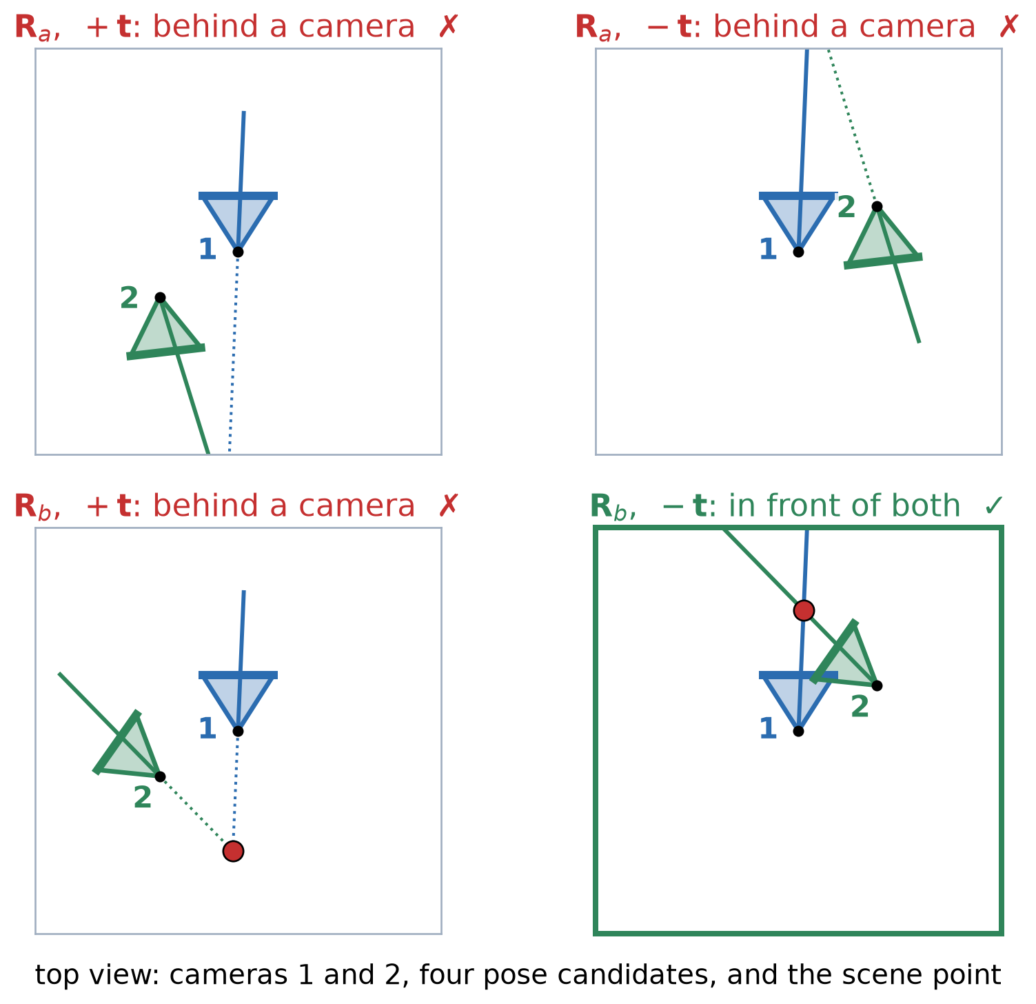
  • \(\mathbf{E} = [\mathbf{t}]_{\times}\mathbf{R}\) can be factored back into \(\mathbf{R}\) and \(\mathbf{t}\)
  • However, this leads to 4 candidate solutions: two rotations, with \(\pm\mathbf{t}\) for each.
  • Only the correct \((\mathbf{R}, \mathbf{t})\) candidate puts the points in front of cameras.
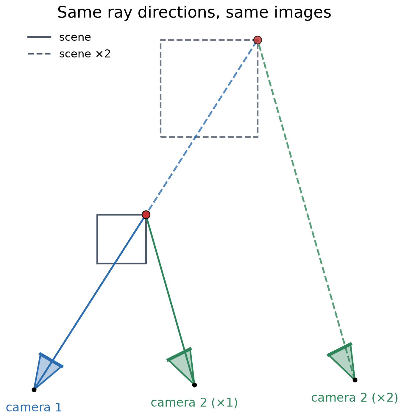
  • Estimated \(\mathbf{t}\) always has unit length: the images cannot tell the scale (a scene twice as large, seen by cameras twice as far apart, gives the same images).
  • For \(\mathbf{F}\): compute \(\mathbf{E} = \mathbf{K}^{\top}\mathbf{F}\,\mathbf{K}\), then the same.
  • For \(\mathbf{H}\) (planar scene): up to 4 candidates \((\mathbf{R},\ \mathbf{t}/d,\ \mathbf{n})\), with the plane normal \(\mathbf{n}\). Requiring the points to be in front of cameras leaves 1 or 2.
  • \(\mathbf{H}\) works for planar scenes, where \(\mathbf{F}\) and \(\mathbf{E}\) are hard to estimate reliably.
Relative Pose With OpenCV

# From E: R, unit-length t, and inlier mask.
n, R, t, mask = cv2.recoverPose(E, pts1, pts2, K)

# From F: convert to E first.
E = K.T @ F @ K

# From H: up to 4 candidates (R, t/d, n).
n, Rs, ts, ns = cv2.decomposeHomographyMat(H, K)
ok = cv2.filterHomographyDecompByVisibleRefpoints(Rs, ns, norm_pts1, norm_pts2)
  • recoverPose tests the 4 candidates and keeps the one with the most points in front of both cameras
  • decomposeHomographyMat decomposes the homography into up to 4 candidates.
  • filterHomographyDecompByVisibleRefpoints keeps only the candidates that are consistent with the visible points in both images.
  • \(\mathbf{E}\) uses \(\mathbf{K}\) during estimation, so it is more accurate than going through \(\mathbf{F}\).

Triangulation: Image Rays Meet at the 3D Point

3D view with orbit slider
view: top behind cameras
  • A pixel \({}^{i}\mathbf{x}\) and its camera define a viewing ray from the camera center \({}^{w}\mathbf{C}_i\) through the pixel on the image plane.
  • Triangulation: with camera poses estimated and \(\mathbf{K}\) known, the two rays meet/intersect at the scene point \({}^{w}\mathbf{X}\), which reconstructs its 3D position in the space.

Noisy Rays Do Not Meet

3D view with orbit slider
view: top behind cameras
  • With pixel noise, the two rays miss each other. Triangulation picks a point \(\hat{\mathbf{X}}\) between them that fits both pixels as well as possible.
  • The reprojection error measures the fit: the distance between each measured pixel and the projection of \(\hat{\mathbf{X}}\).

Depth Precision Depends on Parallax
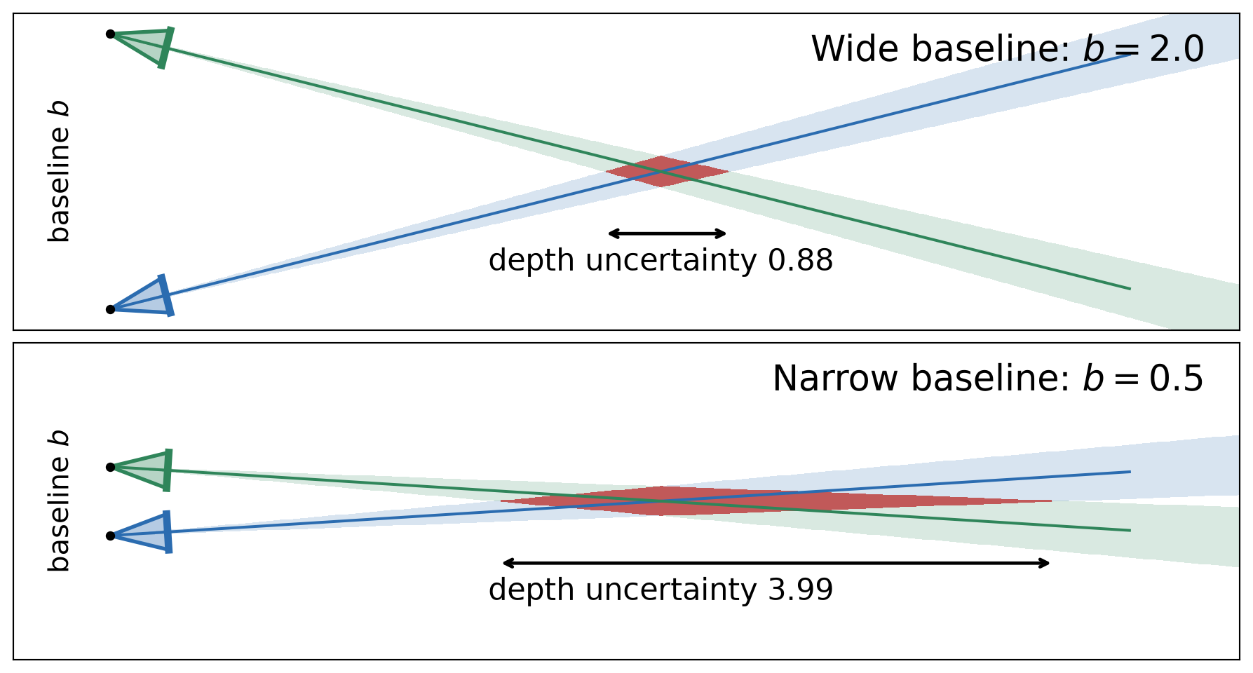
  • Each pixel is uncertain by about a pixel, so each ray is a narrow wedge. The point lies where the two wedges overlap (red).
  • A narrow baseline (little parallax) gives nearly parallel rays: the overlap stretches along the viewing direction, and the depth is uncertain. Far points have the same problem.
  • In the limit of pure rotation (zero baseline), the rays coincide and the depth cannot be found at all.

(Supplementary) Linear Triangulation

  • OpenCV’s cv2.triangulatePoints uses the linear (DLT) method. The steps are:

  • Two rows per camera. Camera \(i\) has projection matrix \(\mathbf{P}_i = \mathbf{K}\,[\mathbf{R}_i \mid \mathbf{t}_i]\) with rows \(\mathbf{p}_{i1}^{\top}, \mathbf{p}_{i2}^{\top}, \mathbf{p}_{i3}^{\top}\). From \(\lambda_i\,{}^{i}\mathbf{x} = \mathbf{P}_i\mathbf{X}\) with \({}^{i}\mathbf{x} = (u_i, v_i, 1)^{\top}\), eliminating \(\lambda_i\) gives two equations, linear in the homogeneous point \(\mathbf{X}\): \[ \big(u_i\,\mathbf{p}_{i3}^{\top} - \mathbf{p}_{i1}^{\top}\big)\,\mathbf{X} = 0, \qquad \big(v_i\,\mathbf{p}_{i3}^{\top} - \mathbf{p}_{i2}^{\top}\big)\,\mathbf{X} = 0 \]

  • Solve. Stack the rows of both cameras into \(\mathbf{A}\) (\(4\times4\)), so \(\mathbf{A}\mathbf{X} = \mathbf{0}\). \(\mathbf{X}\) is the right singular vector of \(\mathbf{A}\) with the smallest singular value; divide it by its fourth entry.

  • Refine (optional). This minimizes an algebraic error. A nonlinear refinement can then minimize the reprojection error in both images.

Triangulation With OpenCV

# Camera matrices K [I | 0] and K [R | t].
P1 = K @ np.hstack([np.eye(3), np.zeros((3, 1))])
P2 = K @ np.hstack([R, t])

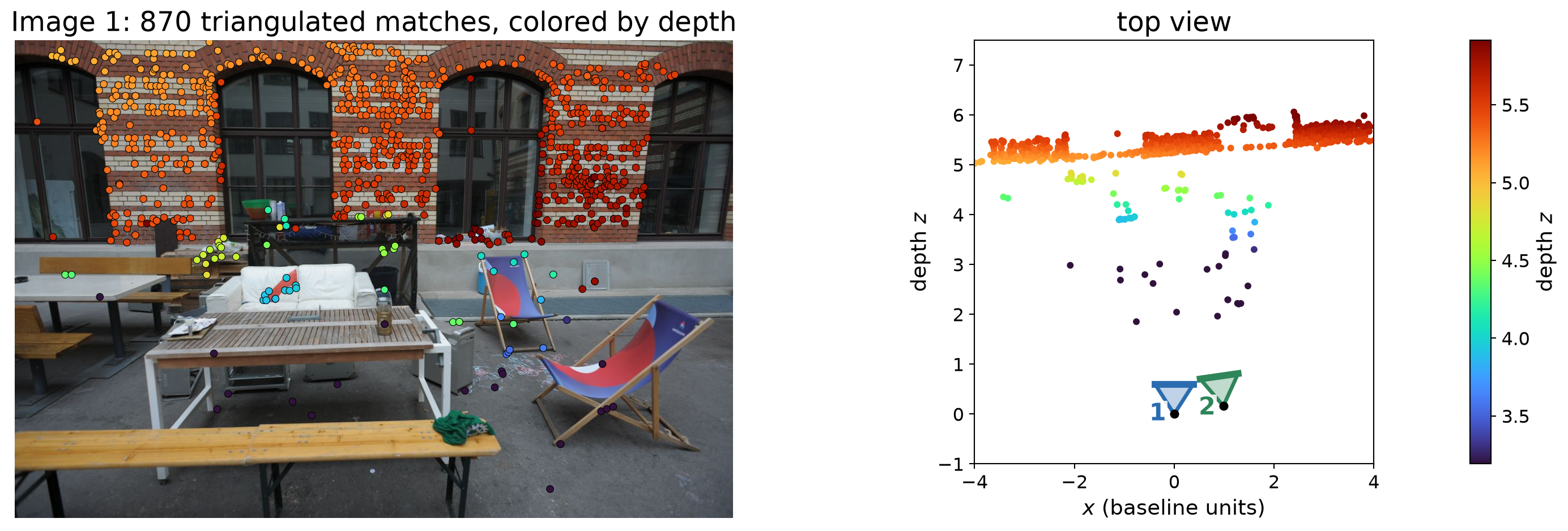
X4 = cv2.triangulatePoints(P1, P2, pts1.T, pts2.T)
X = (X4[:3] / X4[3]).T     # N x 3, camera 1's frame
  • Camera 1 is the reference frame; camera 2 uses the pose from recoverPose.
  • X4 is homogeneous (4×N): divide by its last row.
  • The top view shows the wall as a line behind the table and chairs.

A Denser Reconstruction

  • More points: dense optical flow gives a match for almost every pixel.
  • Keep a match only if its optical flow is consistent forward–backward and lies within 1 px of its epipolar line.
  • Triangulate matches using the recovered pose.
  • The first view is camera 1. The cameras are drawn in blue and green.
  • Holes: surfaces without texture, and parts seen by only one camera.
Point cloud
camera 1 top

Two-View Reconstruction: Full Code

import cv2
import numpy as np

# Two views of the same scene, and the camera intrinsics.
img1 = cv2.imread("assets/13_two_view_geometry/frame1.JPG", cv2.IMREAD_GRAYSCALE)
img2 = cv2.imread("assets/13_two_view_geometry/frame2.JPG", cv2.IMREAD_GRAYSCALE)
K = np.array([[3409.58,    0.0, 3115.16],
              [   0.0, 3409.44, 2064.73],
              [   0.0,    0.0,     1.0]])
K[:2] *= 0.2

# 1. Detect and match features: SIFT with Lowe's ratio test.
sift = cv2.SIFT_create()
kp1, des1 = sift.detectAndCompute(img1, None)
kp2, des2 = sift.detectAndCompute(img2, None)
knn = cv2.BFMatcher(cv2.NORM_L2).knnMatch(des1, des2, k=2)
good = [m for m, n in knn if m.distance < 0.75 * n.distance]
pts1 = np.float32([kp1[m.queryIdx].pt for m in good])
pts2 = np.float32([kp2[m.trainIdx].pt for m in good])

# 2. Essential matrix with RANSAC.
E, mask = cv2.findEssentialMat(pts1, pts2, K, cv2.RANSAC, 0.999, 1.0)

# 3. Relative pose: R and unit t; mask keeps the points in front of both cameras.
n, R, t, mask = cv2.recoverPose(E, pts1, pts2, K, mask=mask)
inliers = mask.ravel() > 0

# 4. Triangulate, with camera 1 as the reference frame.
P1 = K @ np.hstack([np.eye(3), np.zeros((3, 1))])
P2 = K @ np.hstack([R, t])
X4 = cv2.triangulatePoints(P1, P2, pts1[inliers].T, pts2[inliers].T)
X = (X4[:3] / X4[3]).T                    # N x 3, in baseline units

# 5. Depths in each camera (both positive).
depth1 = X[:, 2]
depth2 = (X @ R.T + t.ravel())[:, 2]

print(f"{inliers.sum()} triangulated points")
print("R =\n", R, "\nt =", t.ravel())
print(f"depth range: {depth1.min():.2f} to {depth1.max():.2f} baselines")

Limits of Two-View Reconstruction

  • Scale ambiguity: scaling the scene and the baseline by the same factor gives the same images. A known length (the baseline, an object’s size, GPS, an IMU) is needed for meters.
  • Small parallax: nearly parallel rays give uncertain depths, for far points or a short baseline.
  • Pure rotation gives no depth at all.
  • Matching errors: repeated textures, occlusions, moving objects, and surfaces without texture lead to wrong or missing points.
  • Only what both cameras see is reconstructed. More views add more coverage \(\rightarrow\) structure from motion.
Key Takeaways

  • Epipolar constraint: the match of \({}^{1}\mathbf{x}\) lies on its epipolar line \({}^{2}\ell = \mathbf{F}\,{}^{1}\mathbf{x}\), so \({}^{2}\mathbf{x}^{\top}\mathbf{F}\,{}^{1}\mathbf{x} = 0\). With \(\mathbf{K}\) known, \(\mathbf{E} = \mathbf{K}^{\top}\mathbf{F}\,\mathbf{K} = [\mathbf{t}]_{\times}\mathbf{R}\).
  • \(\mathbf{F}\) needs 7 or 8 matches; \(\mathbf{E}\) needs 5 (and \(\mathbf{K}\)). Some matches are always wrong, so estimate with RANSAC: fit minimal samples, keep the model with the most inliers, refit.
  • Homography: \({}^{2}\mathbf{x} = \mathbf{H}\,{}^{1}\mathbf{x}\) maps a point to a point, but only for a planar scene, a rotating camera, or a distant scene.
  • Relative pose: \(\mathbf{E}\) (or \(\mathbf{H}\)) gives up to 4 \((\mathbf{R}, \mathbf{t})\) candidates; keep the one with the points in front of cameras. \(\mathbf{t}\) is known only up to scale.
  • Triangulation intersects the two viewing rays. With noise they miss, so pick the point with the smallest reprojection error. Accurate depth needs enough parallax (baseline).
  • In OpenCV: findEssentialMat → recoverPose → triangulatePoints; findFundamentalMat and findHomography for the uncalibrated and planar cases.