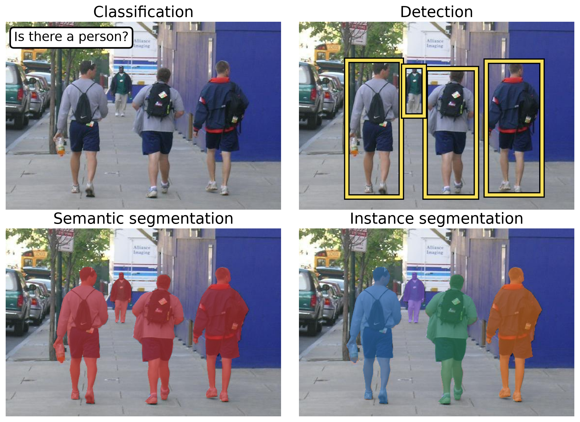
Lecture 15 — Machine Learning for Computer Vision
Lecture 15
Why Is Recognition Hard?
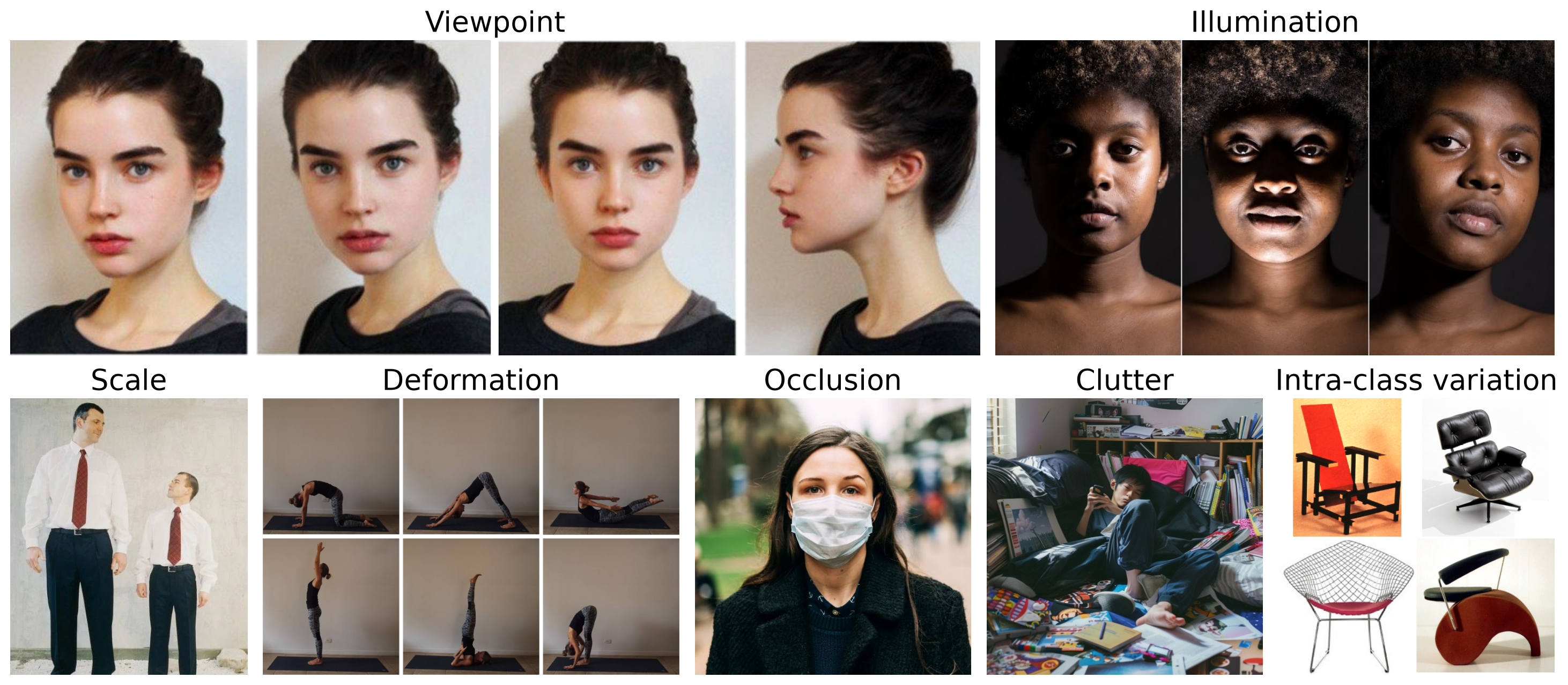
- How many different object classes are there? Roughly 10,000 to 30,000.
- Objects of the same class can have very different pixels.
The Data-Driven Approach
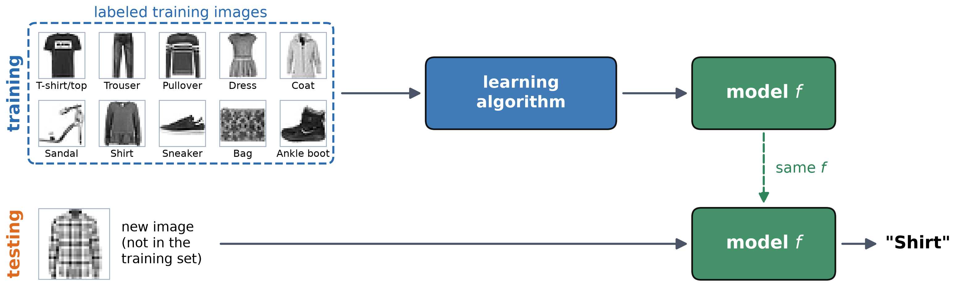
- Training set: Images with ground truth labels.
- Learning: A learning algorithm fits a model \(f\) to data: \(f(\text{image}) \approx \text{label}\).
- Inference: Use \(f\) on new images. What matters is how well \(f\) does on images it has never seen.
Types of Learning
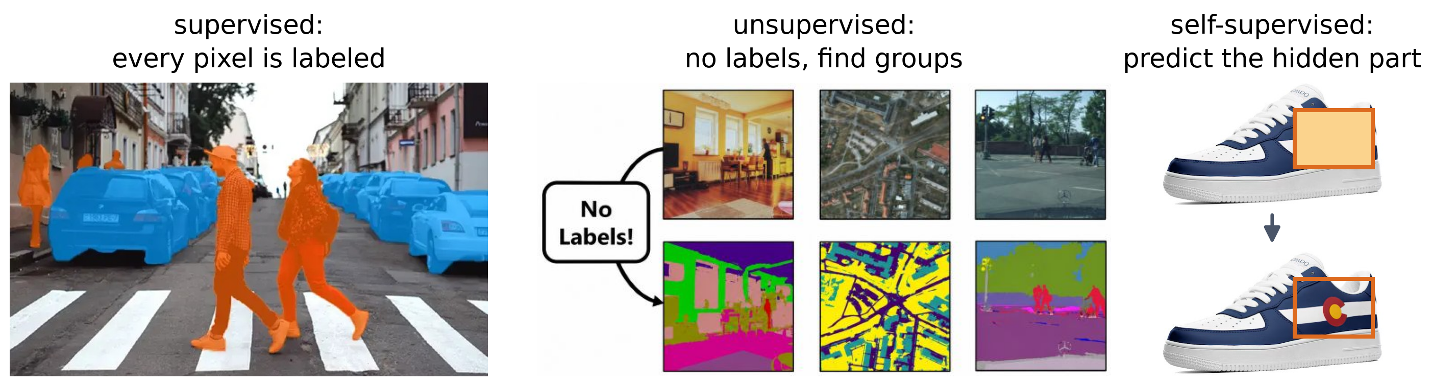
| Type | Training data | Vision examples |
|---|---|---|
| Supervised | images and labels | classify clothing; detect pedestrians |
| Unsupervised | images only | group pixels by color (clustering); compress images (PCA) |
| Self-supervised | images only; the labels come from the data itself | predict hidden patches; match images to their captions |
- Labels cost effort, more so for richer labels: tag < box < mask.
Common Machine Learning Datasets for Computer Vision

| Dataset | Year | Images | Classes | Image size | Task |
|---|---|---|---|---|---|
| MNIST | 1998 | 60,000 train + 10,000 test | 10 digits | 28 × 28, gray | classification |
| FashionMNIST | 2017 | 60,000 train + 10,000 test | 10 clothing types | 28 × 28, gray | classification |
| CIFAR-10 | 2009 | 50,000 train + 10,000 test | 10 objects and animals | 32 × 32, color | classification |
| ImageNet | 2012 | 1.28 M train + 50,000 val | 1,000 | varies, color | classification |
| COCO | 2014 | 118,000 train + 5,000 val | 80 | varies, color | detection, segmentation, captions |
| Penn-Fudan | 2007 | 170 | pedestrians | varies, color | detection, segmentation |
- These are benchmarks that are widely used to compare methods on the same data.
- ImageNet’s size made deep learning practical (2012).
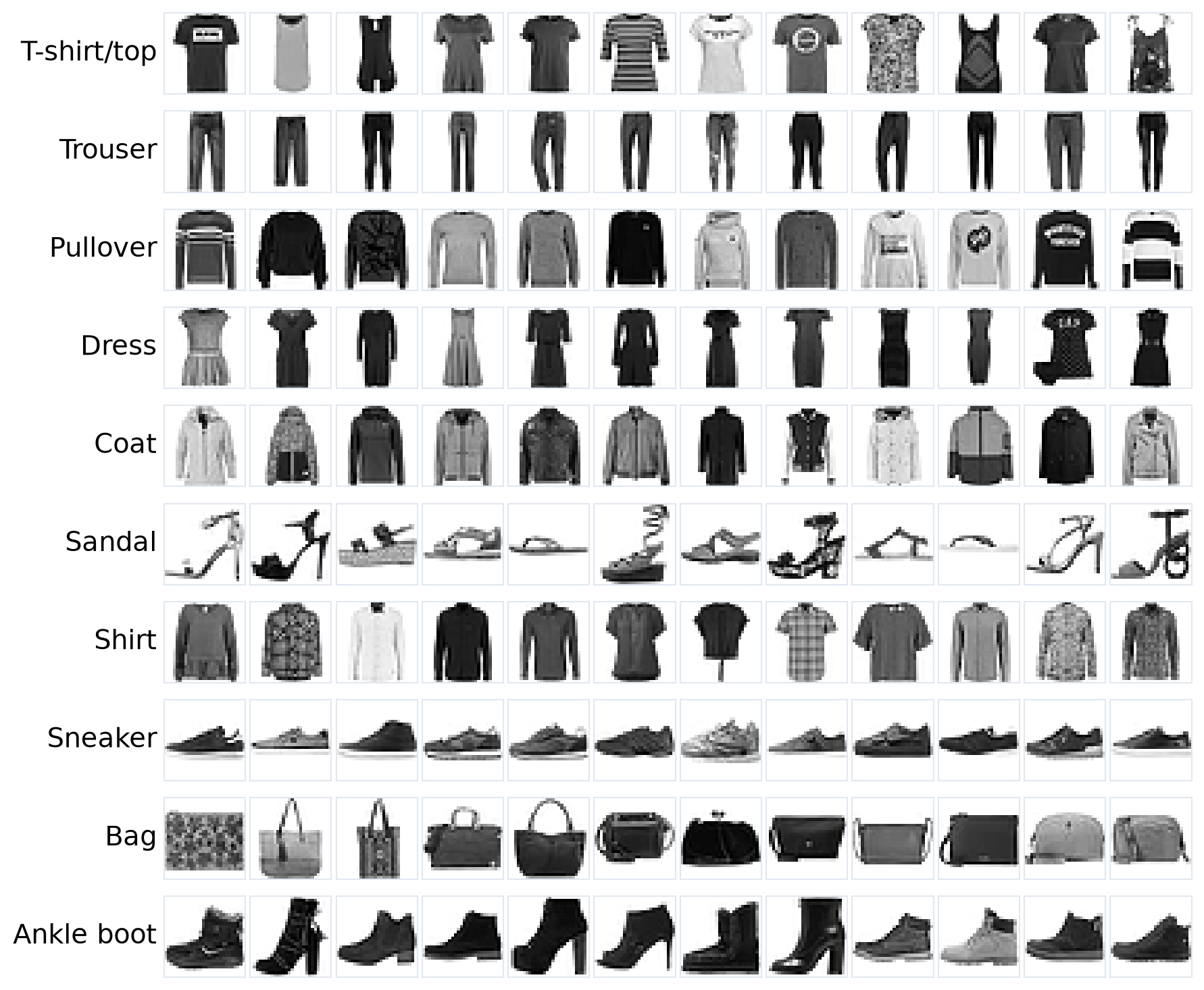
FashionMNIST: Our Running Example
| Images | Per class | |
|---|---|---|
| Training | 60,000 | 6,000 |
| Test | 10,000 | 1,000 |
28 × 28 gray images: 784 pixels, values 0 to 255.
Same format as MNIST, but harder: T-shirt, pullover, coat, and shirt look alike.
Small enough to train on a laptop CPU.
We compare our classifiers on this benchmark.
A Toy Learning Problem
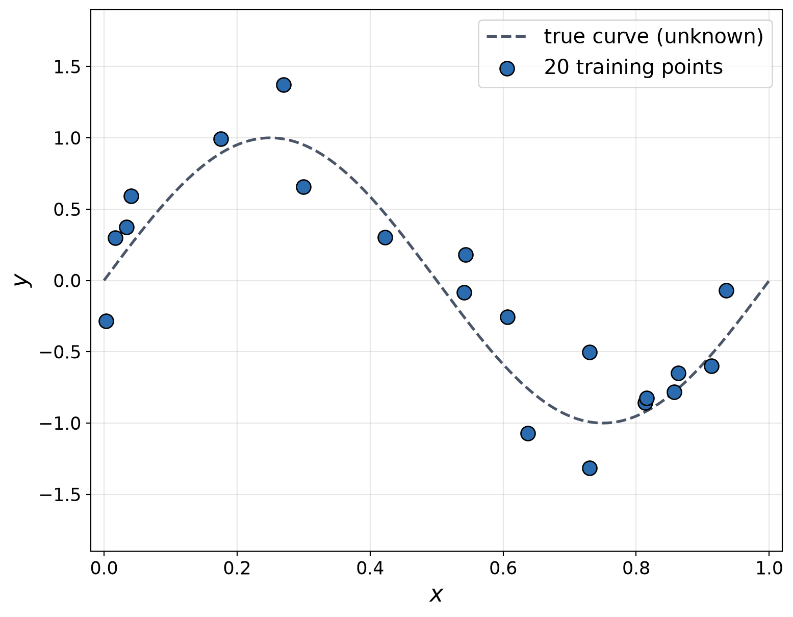
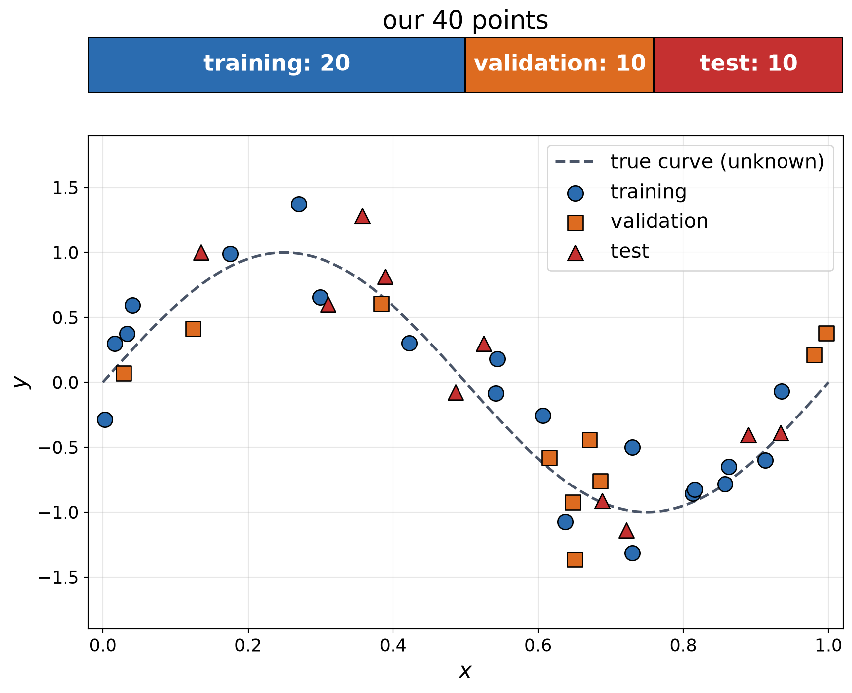
- Task: predict \(y\) from \(x\), using only the noisy points.
- Model: a polynomial of degree \(M\):
\[ \bbox[border: 2px solid #c53030; padding: 2px 6px]{\hat{y} = w_0 + w_1 x + w_2 x^2 + \dots + w_M x^M}\;\;{\color{#c53030}{\begin{array}{l}\textbf{polynomial}\\ \textbf{model}\end{array}}} \]
- \(x\): input; \(\hat{y}\): prediction
- \(w_0, \dots, w_M\): parameters learned from the data.
- Learning: pick the \(w\)’s with the smallest mean squared error (MSE) on the training points:
\[ \text{MSE} = \frac{1}{N} \sum_{i=1}^{N} \left(y_i - \hat{y}_i\right)^2 \]
- \(y_i\): true value; \(\hat{y}_i\): prediction for point \(i\); \(N\): number of points.
Model Complexity: Underfitting vs. Overfitting
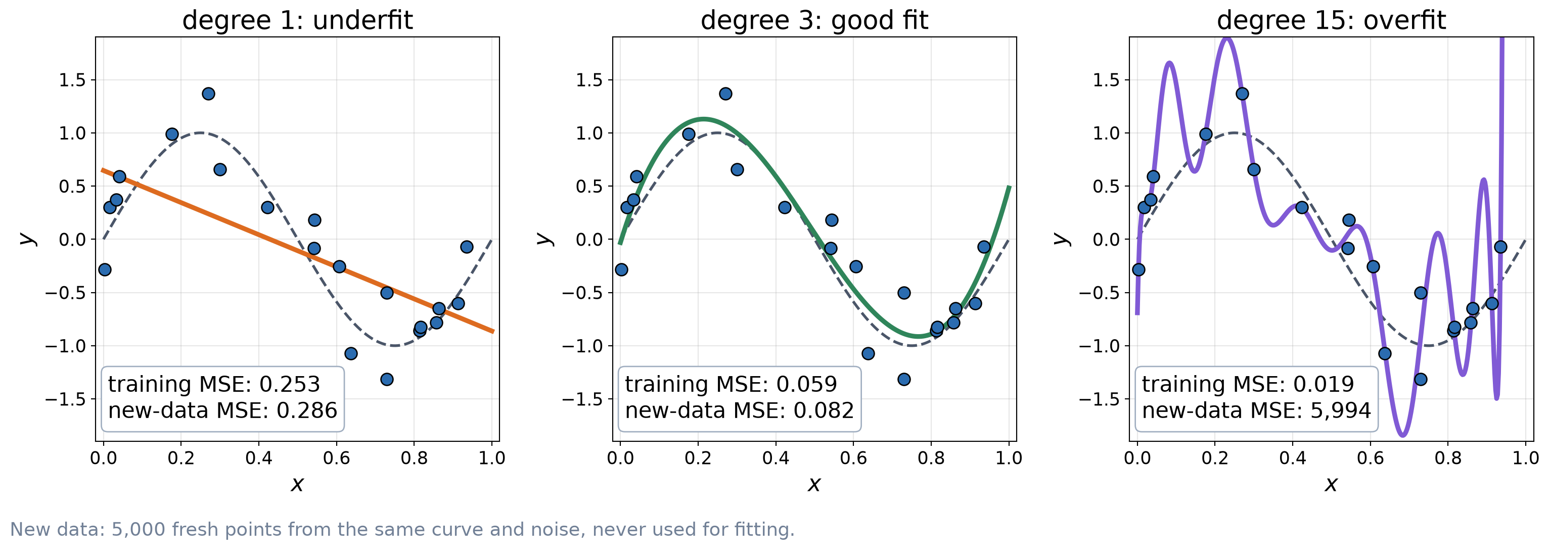
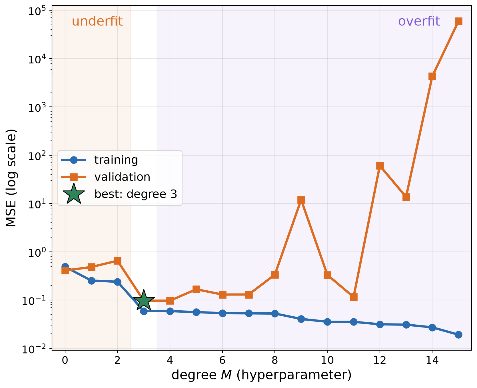
- Underfit: too simple to follow the pattern \(\rightarrow\) high error everywhere.
- Overfit: so flexible that it fits the noise \(\rightarrow\) lowest training error, huge error on new data.
- The goal is generalization: low error on data the model has not seen. Training error alone does not tell us that.
Train / Validation / Test
- Training set: fit the parameters \((w_0, \dots, w_M)\).
- Validation set: choose the hyperparameters: settings we pick, not learned (here, the degree \(M\)).
- Test set: measure the final error once, at the end. Never use it to make choices.
Choosing the Degree
Choosing a Hyperparameter
- For each candidate \(M\): fit on the training set.
- Measure the error on the validation set.
- Keep the \(M\) with the lowest validation error.
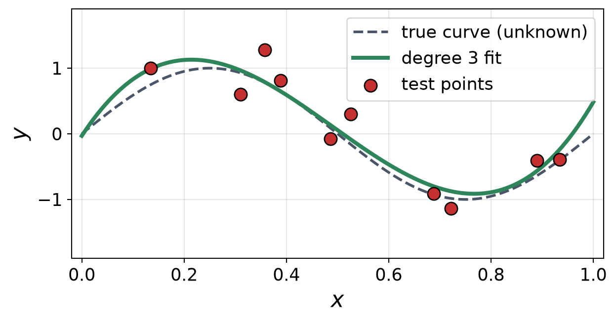
- Report the test error of that model, once.
- Training error keeps falling as \(M\) grows. Validation error falls, then rises.
- Best: \(M\) = 3 (validation MSE 0.097). Its test MSE: 0.072.
Bias–Variance Trade-Off
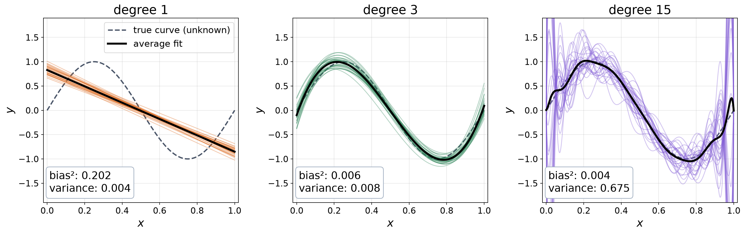
- Each thin line: a fit to a different training set (same \(x\), new noise). Black: their average.
- Bias: the average fit misses the truth \(\rightarrow\) the model is too simple.
- Variance: the fit changes a lot from one training set to the next \(\rightarrow\) the model is too flexible.
- New-data error \(\approx\) bias² + variance + noise. The best complexity balances the two.
More Data Helps

- With few points, the flexible model fits the noise. With many, it cannot fit the noise, so it follows the true curve.
- Training and new-data errors meet at the noise level, which no model can beat.
- More data is often the best cure for overfitting.
Polynomial Fitting in Code
Polynomial.fit(x, y, deg): finds the \(w\)’s with the smallest training MSE (least squares).model(x): evaluates the fitted polynomial atx.mse(...): the mean squared error from before.min(val_mse, key=val_mse.get): the degree with the lowest validation error.
On our data: best \(M\) = 3, test MSE = 0.072.
import numpy as np
from numpy.polynomial import Polynomial
def mse(model, x, y):
return np.mean((model(x) - y) ** 2)
# (x_tr, y_tr), (x_val, y_val), (x_te, y_te): splits
val_mse = {}
for M in range(16):
model = Polynomial.fit(x_tr, y_tr, deg=M)
val_mse[M] = mse(model, x_val, y_val)
best_M = min(val_mse, key=val_mse.get)
model = Polynomial.fit(x_tr, y_tr, deg=best_M)
print(best_M, mse(model, x_te, y_te)) # test: onceEvaluation Metrics Depend on the Task
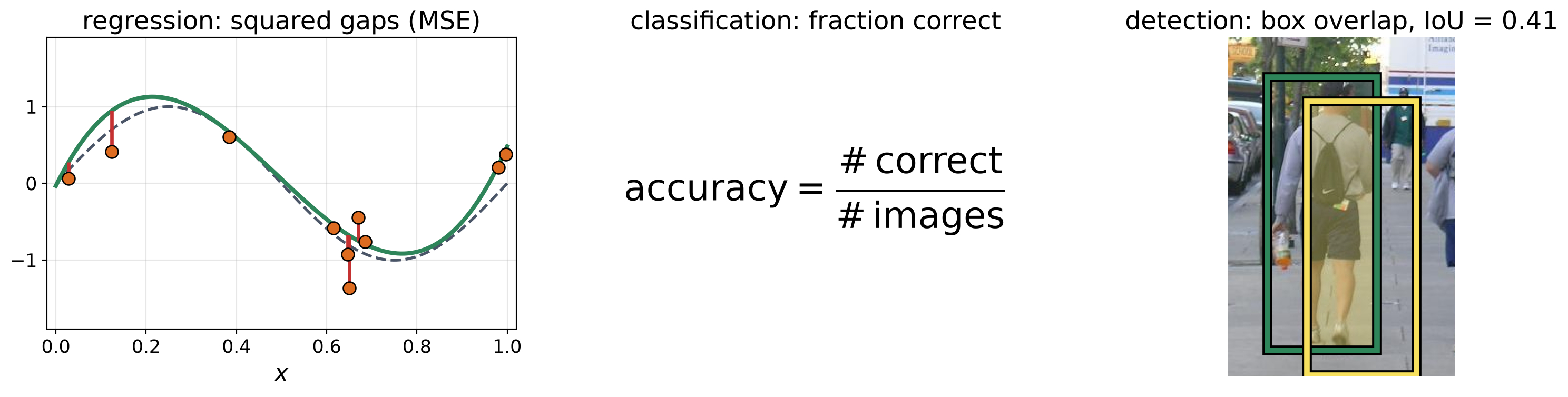
| Task | Output | Common metrics |
|---|---|---|
| Regression | number(s) | mean squared error (MSE) |
| Classification | a category | accuracy; confusion matrix (which classes get mixed up) |
| Detection | a box and class per object | intersection over union (IoU); precision and recall; average precision (AP) |
| Segmentation | a label per pixel | IoU per class |
When Accuracy Misleads
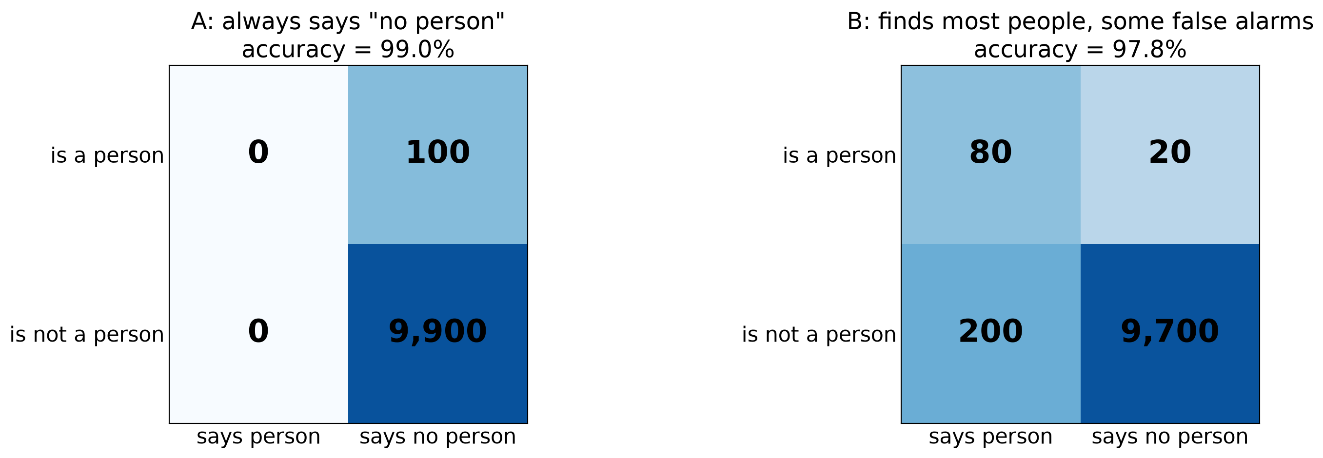
- 10,000 images, only 1% contain a person. Method A finds nobody, yet has a higher accuracy than method B that finds most people (99.0% vs. 97.8%).
- Need to look at both precision and recall. Precision: fraction of correct detections (A: undefined (no detections), B: 29%). Recall: fraction of people found (A: 0%, B: 80%).
- Accuracy is fine when the classes are balanced (as in FashionMNIST).
An Image Is a Vector
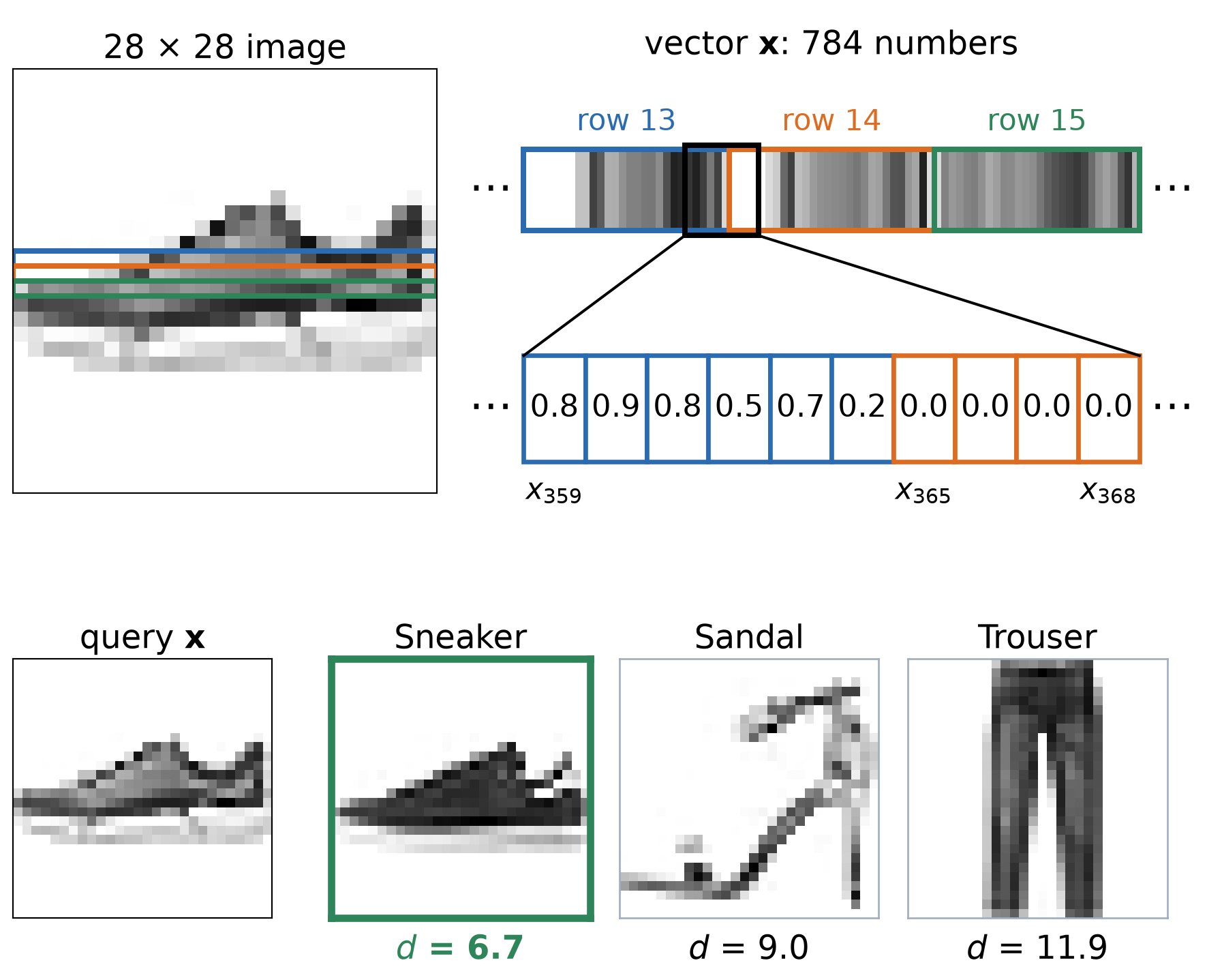
- A 28 × 28 gray image is 784 numbers. Stack its rows into one long vector \(\mathbf{x} = (x_1, x_2, \dots, x_{784})\).
- Compare two images pixel by pixel:
\[ \bbox[border: 2px solid #c53030; padding: 2px 6px]{d(\mathbf{x}, \mathbf{x}') = \sqrt{\sum_{j=1}^{784} \left(x_j - x'_j\right)^2}}\;\;{\color{#c53030}{\begin{array}{l}\textbf{L2}\\ \textbf{distance}\end{array}}} \]
- \(x_j\), \(x'_j\): value of pixel \(j\) (0 to 1) in images \(\mathbf{x}\) and \(\mathbf{x}'\).
- Small \(d\): similar images. Large \(d\): different images.
- The sneaker is closest to the other sneaker (\(d\) = 6.7) and farthest from the trouser (\(d\) = 11.9).
Examples of Nearest Neighbors on FashionMNIST
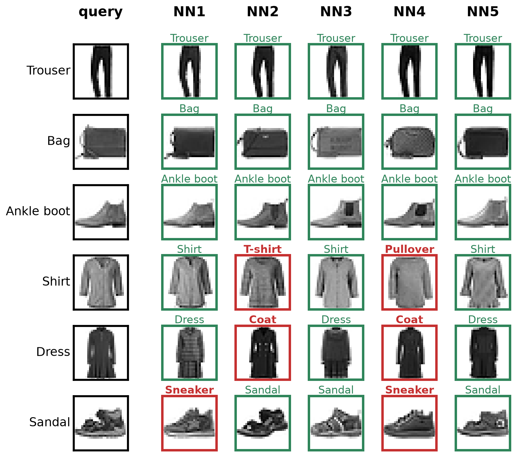
- Query (left column): a test image.
- Neighbors: the 5 training images with the smallest L2 distance to the query, from NN1 (closest) to NN5.
- Green frame: same class as the query. Red frame: a different class.
- Mistakes come from look-alike classes: the shirt has T-shirt and pullover neighbors, and the dress has coat neighbors.
- The sandal’s closest neighbor is a sneaker, but 3 of its 5 neighbors are sandals.
- Simple idea: classify a new image based on the majority class among its \(k\) nearest neighbors.
k-Nearest Neighbors (KNN) Classification
k-Nearest Neighbors (KNN)
Training: store all training images and their labels.
Prediction for a new image \(\mathbf{x}\):
- Compute the distance from \(\mathbf{x}\) to every training image.
- Find the \(k\) closest training images.
- Predict the most common label among them (majority vote).
- 2D points represent images: each point is a vector with 2 numbers instead of 784.
- Small \(k\): one noisy neighbor decides.
- Large \(k\): far-away points join, and the big class wins.

Decision Boundaries Change with k
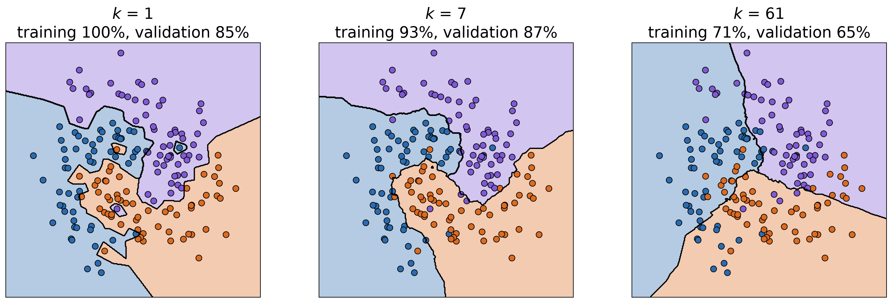
- Decision boundary: where the predicted class changes. Each location is colored by its KNN prediction.
- Small \(k\): jagged boundary with islands around single points. It fits the noise (overfitting).
- Large \(k\): smooth boundary, but the arms of the spiral get washed out (underfitting).
- \(k\) is a hyperparameter: choose it on validation data, like the polynomial degree.
Choosing k on FashionMNIST
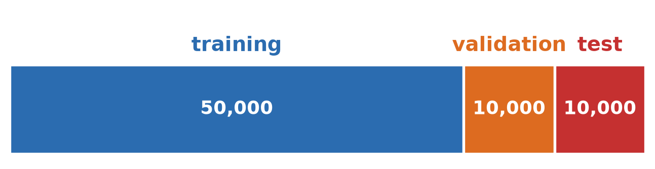
- Split the 60,000 training images: 50,000 training + 10,000 validation. Keep the 10,000 test images aside.
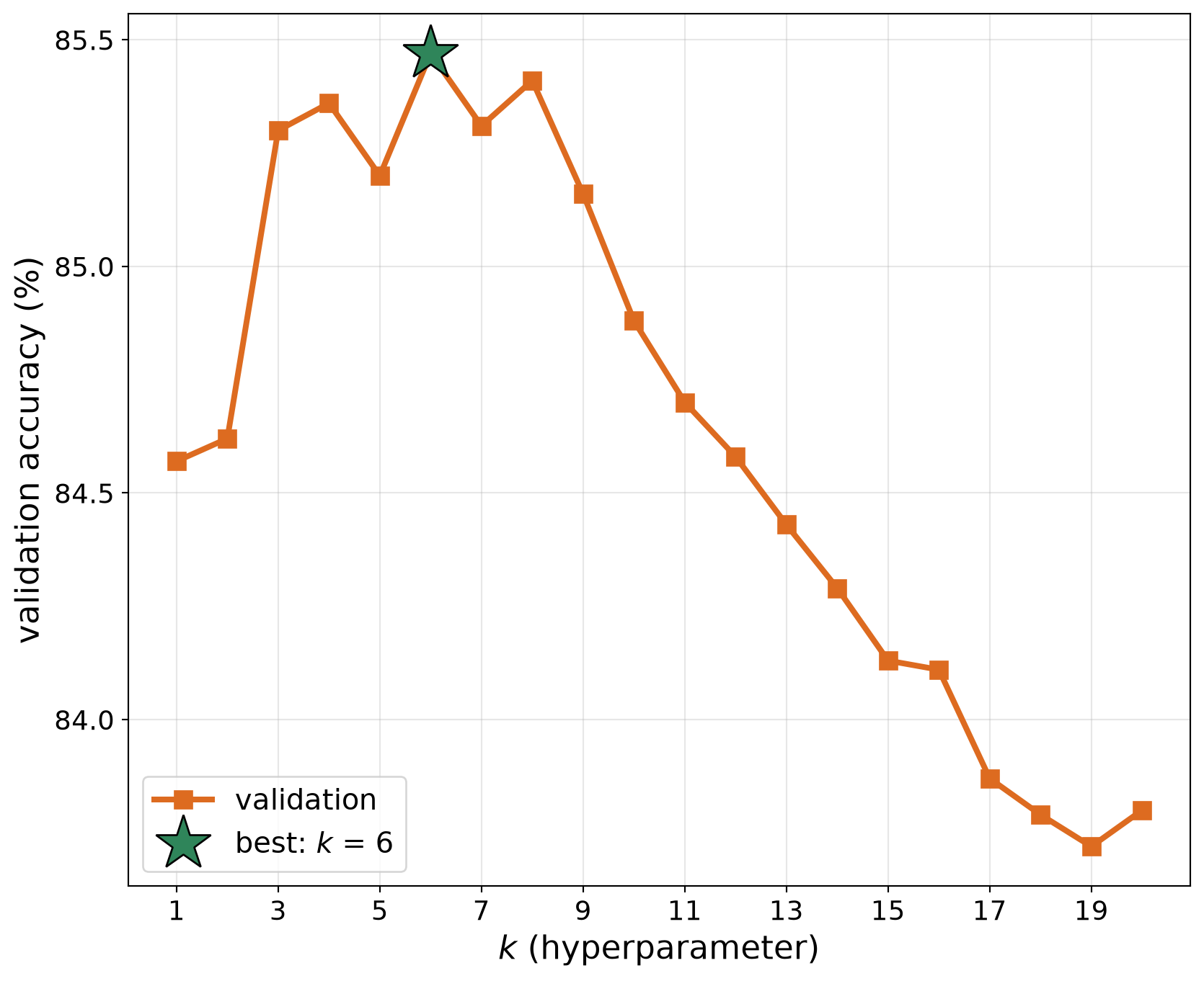
- Same recipe as choosing the polynomial degree: for each \(k\) = 1, …, 20, predict the validation images with KNN and measure the accuracy.
- Best: \(k\) = 6 (validation accuracy 85.5%).
- Test accuracy with \(k\) = 6, measured once: 85.0%.
KNN in Code
KNearest_create(): an empty KNN model.train(X, cv2.ml.ROW_SAMPLE, y): stores the data.X: one image per row (float32);y: the labels.findNearest(X, k): KNN prediction for each row ofX. Returns the predicted labels, the labels of thekneighbors, and their distances.
- On our data (\(k\) = 6): test accuracy 85.0%, about 1 ms per test image.
import cv2
import numpy as np
# X_tr: (50000, 784) float32, y_tr: labels 0-9
# X_te: (10000, 784) float32, y_te: labels 0-9
knn = cv2.ml.KNearest_create()
knn.train(X_tr, cv2.ml.ROW_SAMPLE,
y_tr.astype(np.float32))
# best_k: chosen on the validation set
_, pred, neighbors, dist = knn.findNearest(
X_te, k=best_k)
pred = pred.ravel().astype(int)
print("test accuracy:", np.mean(pred == y_te))
Confusion Matrix and Accuracy
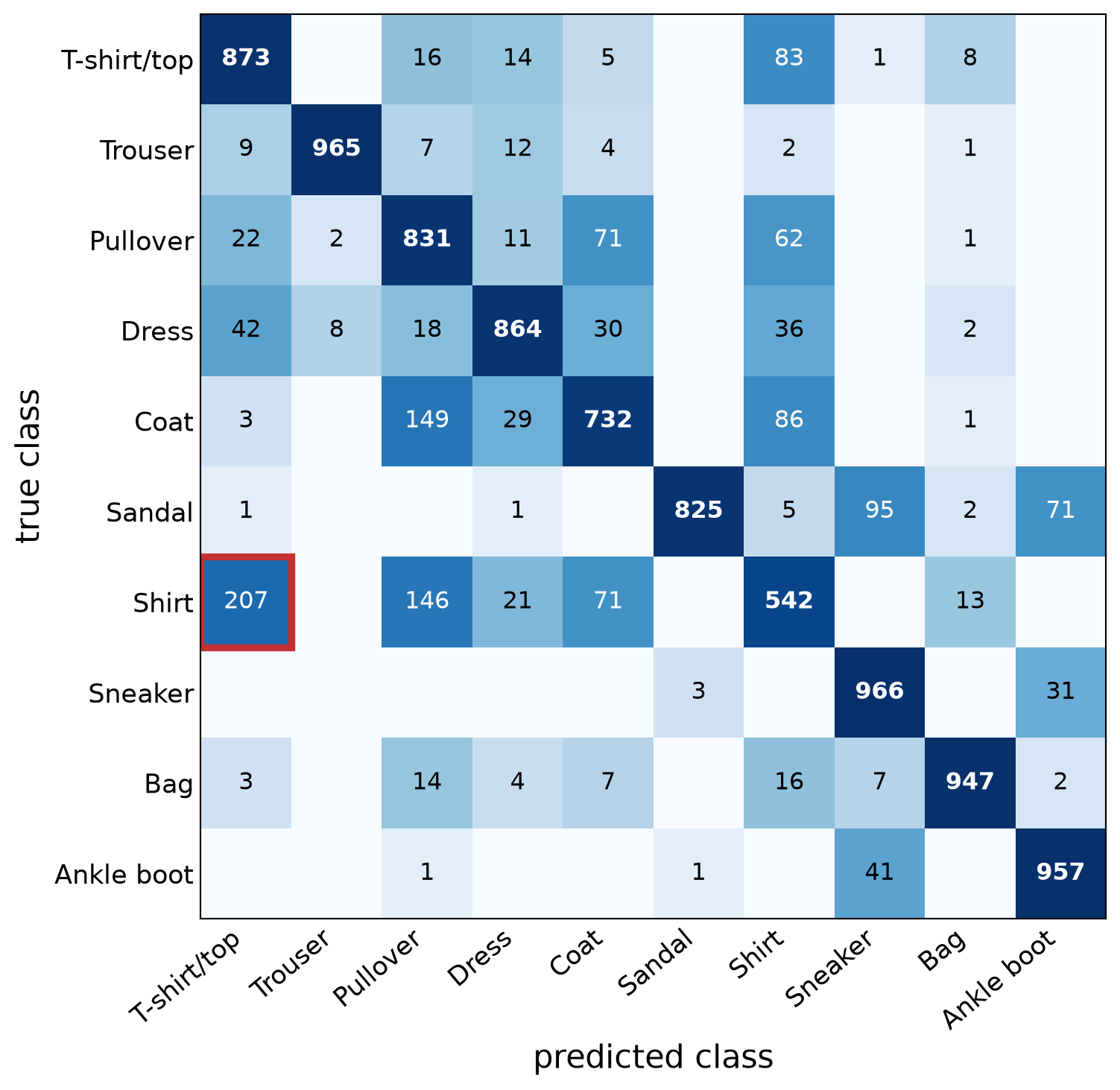
Confusion matrix: entry (row \(i\), column \(j\)) = number of test images of class \(i\) predicted as class \(j\).
Diagonal: correct predictions. Off-diagonal: mistakes, and which classes get mixed up.
\(\text{accuracy} = \dfrac{\text{sum of the diagonal}}{\text{sum of all entries}}\)
KNN (\(k\) = 6): 8,502 / 10,000 correct = 85.0%.
Easiest: Sneaker (97% correct). Hardest: Shirt (54%), most often called T-shirt/top (207 times).
Limitations of KNN
- Slow prediction: compares each new image with all 50,000 training images (about 1.4 ms per new image on a CPU, for all 50,000 comparisons).
- Stores all the data: 50,000 × 784 values = 157 MB. More data: more memory and slower predictions.
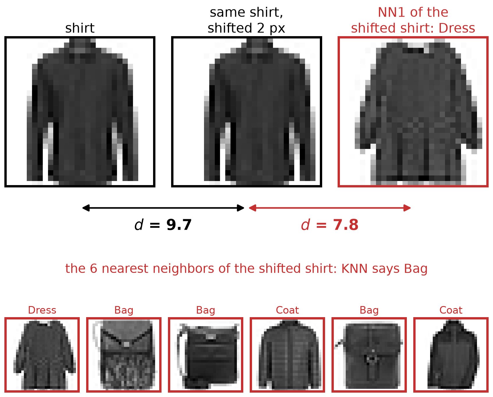
- Pixel distance is not semantic: a 2-pixel shift is invisible to us, but changes many pixels.
- The shifted shirt is 9.7 away from the original, but a dress is only 7.8 away.
- Shifting all test images by 2 pixels drops the accuracy from 85.0% to 67.0%.
- Next: better features and better classifiers.
k-Means Clustering
- Unsupervised: points without labels. Goal: group them into \(k\) clusters of nearby points.
- Each cluster has a center. Each point belongs to the nearest center.
k-Means Clustering
- Pick \(k\) starting centers (e.g., \(k\) random points).
- Assign: each point joins its nearest center.
- Update: move each center to the mean of its points.
- Repeat 2–3 until the assignments stop changing.
- \(k\) is a hyperparameter.
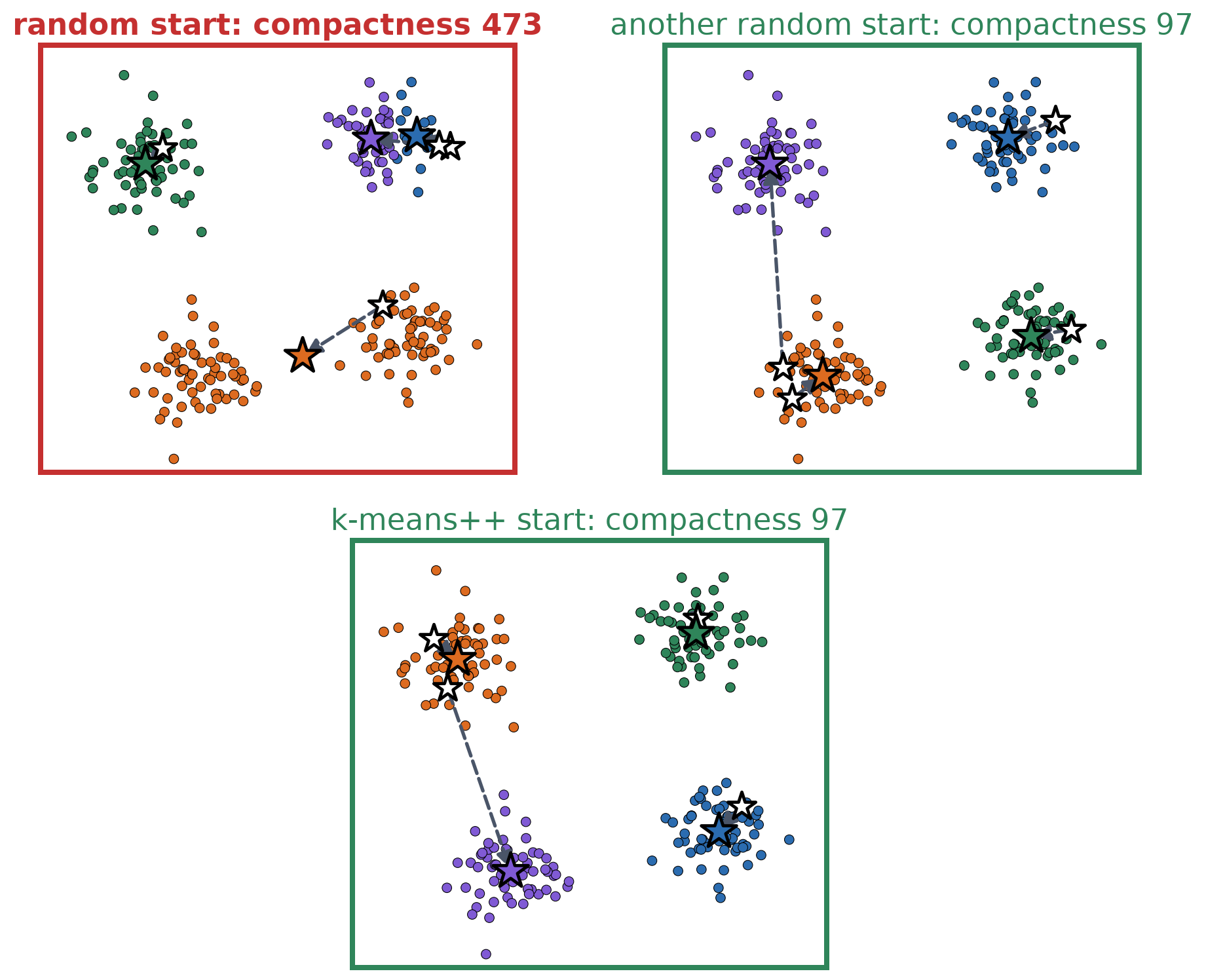
- Different starting centers can lead to different final clusters.

Starting Centers Matter
- A bad start can get stuck in a bad result (top left: two blobs share one center; white stars: starting centers; colored stars: final centers).
- Compactness: sum of squared distances from each point to its center. Lower is better.
- Several attempts: run from different starts; keep the lowest compactness.
- k-means++: first center at random; each next center far from the chosen ones.
Color Segmentation with k-Means
- Each pixel is a point \((R,G,B)\) in 3D color space.
- k-means with \(k\) clusters groups the pixels into \(k\) groups, each represented by a color (the center).
- Pixels of similar color land in one cluster, even on different objects.
- No labels needed: the colors group by themselves.

PCA: The Directions of Largest Variance
- PCA (principal component analysis): find the directions in which the data varies the most.
PCA
- Subtract the mean from every point.
- First component \(\mathbf{u}_1\): the direction of largest variance.
- Next components \(\mathbf{u}_2, \mathbf{u}_3, \dots\): largest remaining variance, perpendicular to the previous ones.
- Keep the first \(k\). Describe each point by its \(k\) coordinates along them.
- The components are the eigenvectors of the data’s covariance matrix.
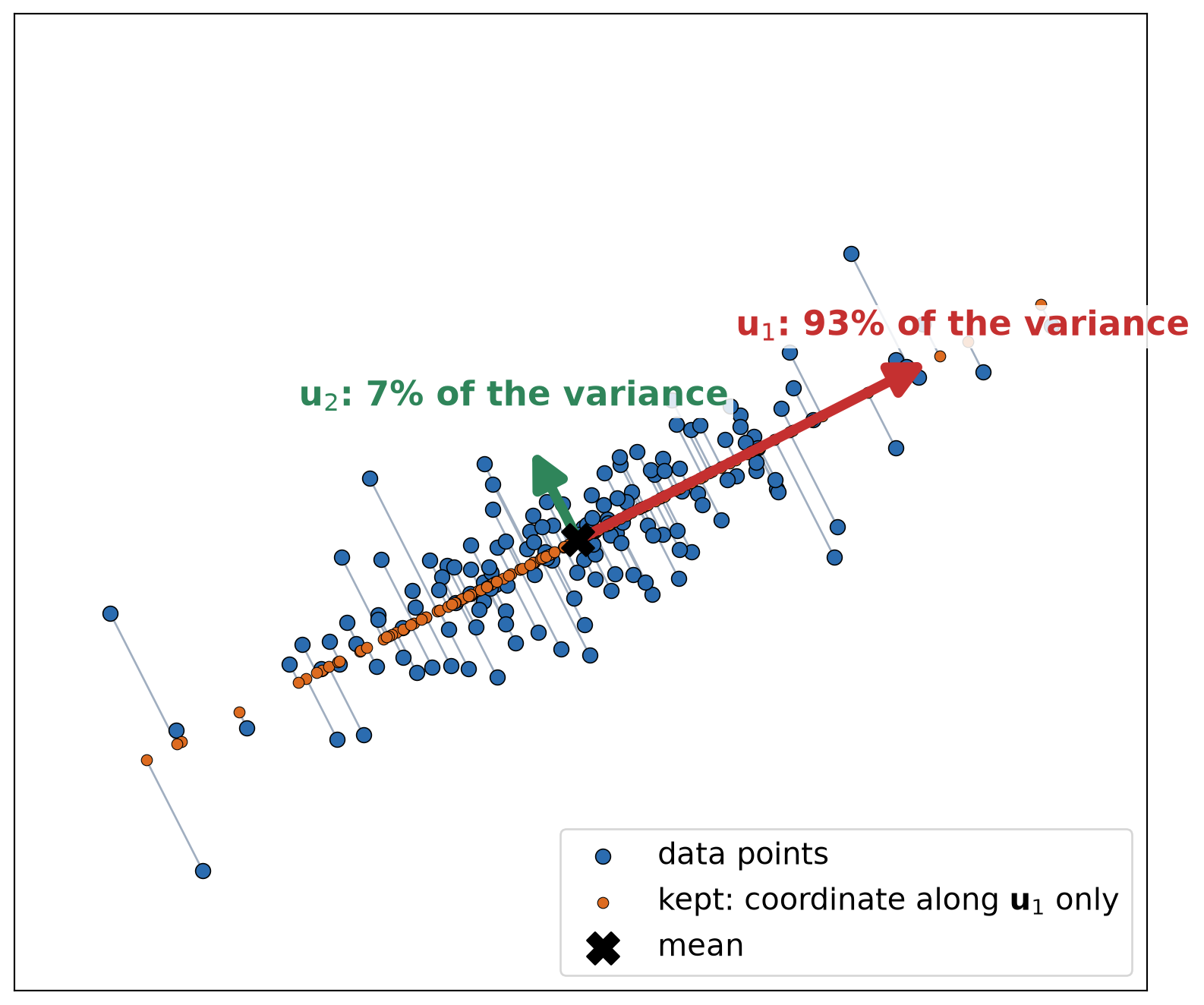
\(\mathbf{u}_1\) holds 93% of the variance. Keep only the coordinate along \(\mathbf{u}_1\): 1 number instead of 2, and the points barely move.
PCA on FashionMNIST
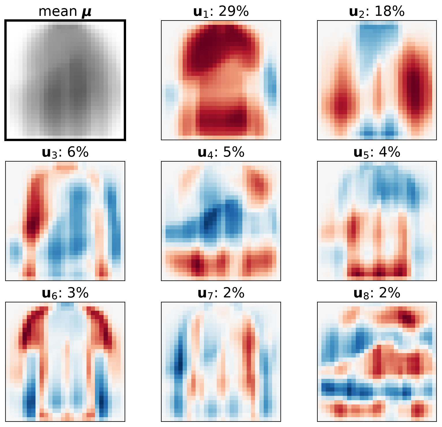
- PCA of the 50,000 training images, each a vector of 784 numbers.
- Mean image \(\boldsymbol{\mu}\) and components \(\mathbf{u}_j\) are 784-vectors too: show them as images.
- Red: add ink to the mean. Blue: remove ink. Early components: coarse shapes. Later: finer details.
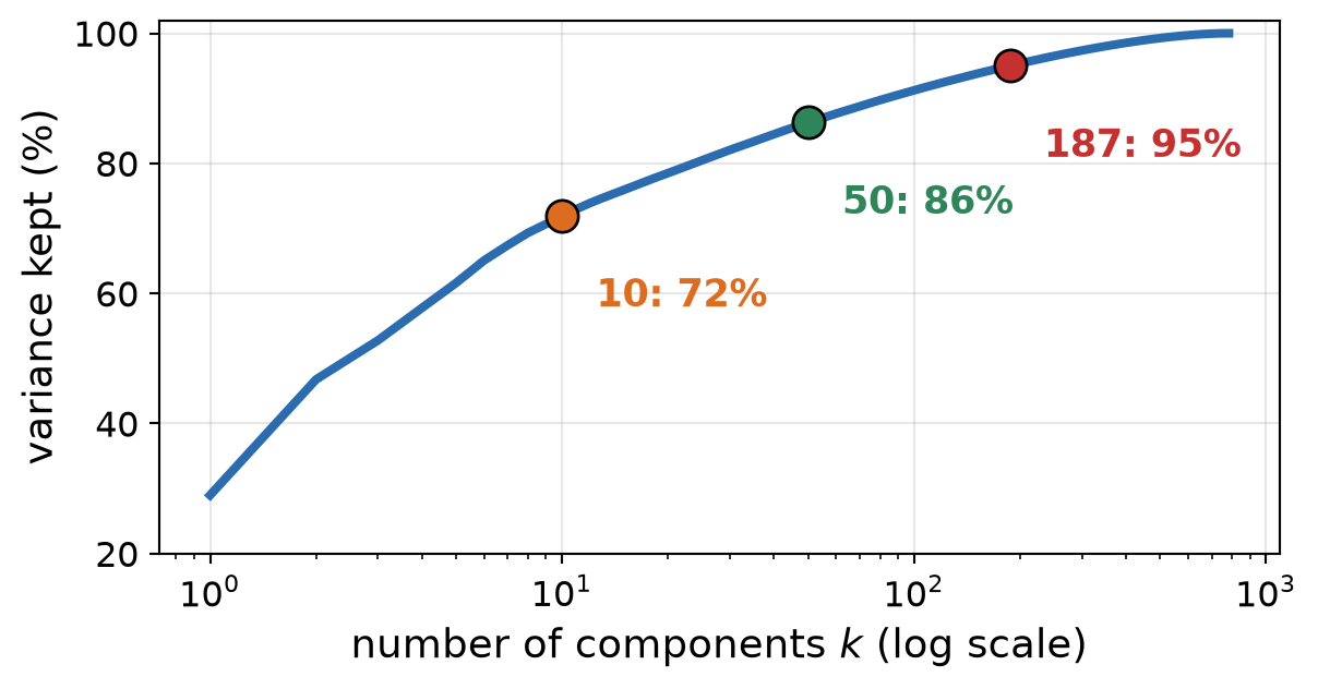
- Variance kept: 72% with 10 components, 86% with 50. 187 of the 784 components keep 95%.
Reconstruction with k Components
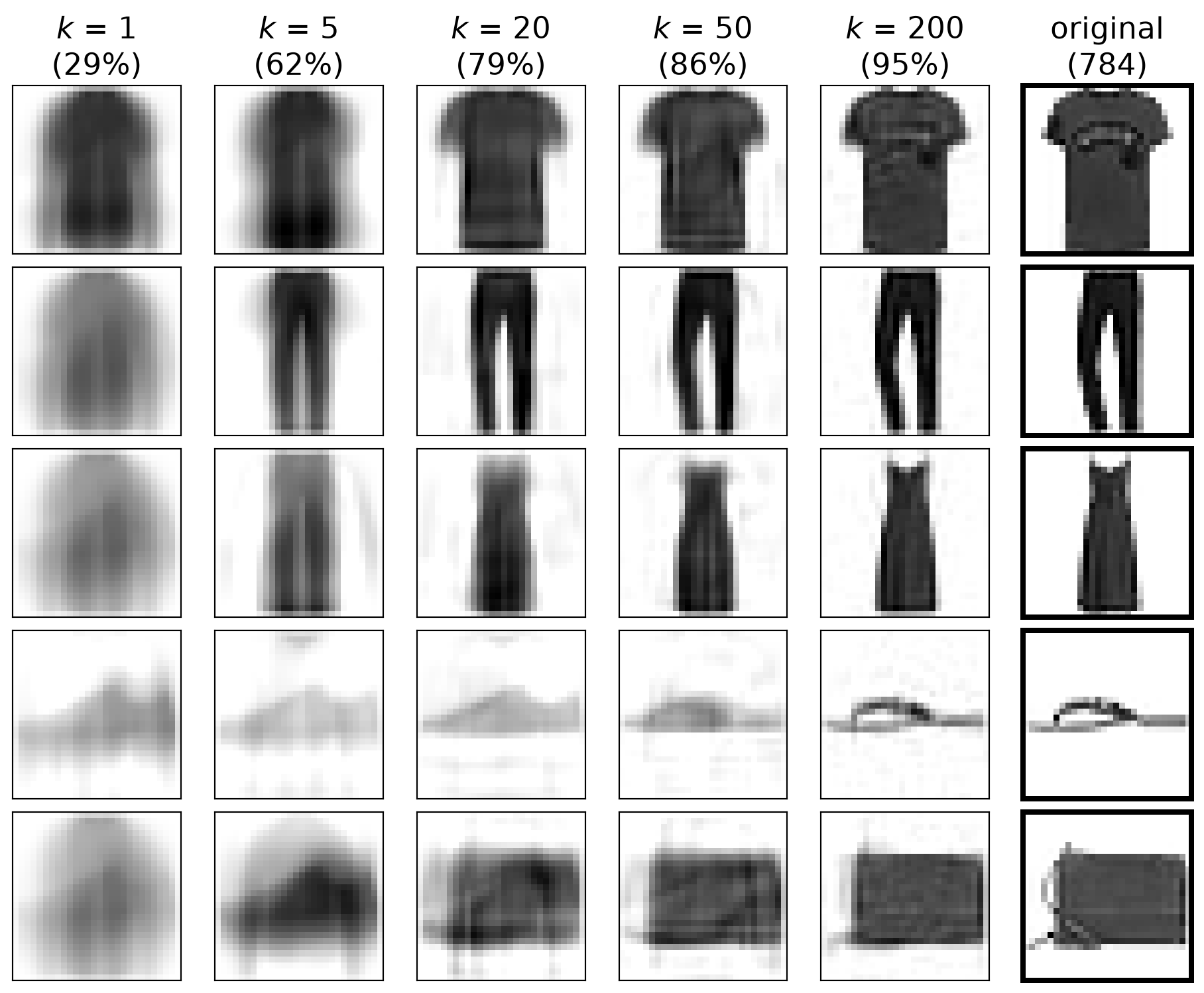
- Any image is the mean plus a weighted sum of components:
\[ \bbox[border: 2px solid #c53030; padding: 2px 6px]{\hat{\mathbf{x}} = \boldsymbol{\mu} + a_1 \mathbf{u}_1 + \dots + a_k \mathbf{u}_k}\;\;{\color{#c53030}{\begin{array}{l}\textbf{PCA}\\ \textbf{reconstruction}\end{array}}} \]
- \(\boldsymbol{\mu}\): mean image; \(\mathbf{u}_j\): component \(j\).
- \(a_j = \mathbf{u}_j \cdot (\mathbf{x} - \boldsymbol{\mu})\): coordinate of image \(\mathbf{x}\) along \(\mathbf{u}_j\).
- With \(k\) = 50 numbers instead of 784, the garment is still easy to recognize.
- So the coordinates \((a_1, \dots, a_k)\) are compact features: an input for a classifier.
PCA Features for Recognition
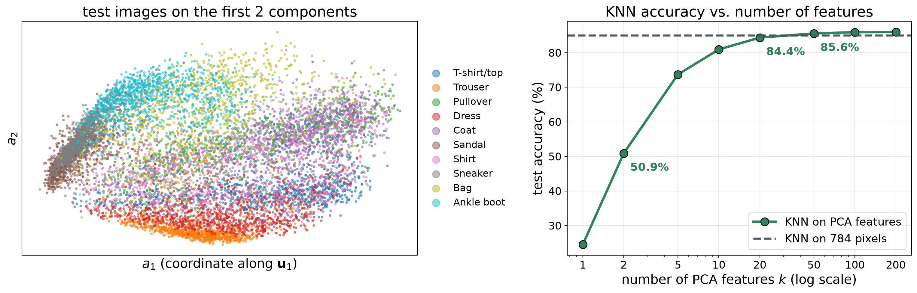
- Left: PCA uses no labels, yet with 2 numbers per image many classes form their own regions; look-alike classes overlap.
- Right: 20 features: within 1 point of the 784 pixels (84.4% vs. 85.0%). From 50 on, slightly better (the small components are mostly pixel noise).
- Still pixel-based: a 2-pixel shift drops KNN on 50 PCA features to 66.0%.
Linear Classifiers
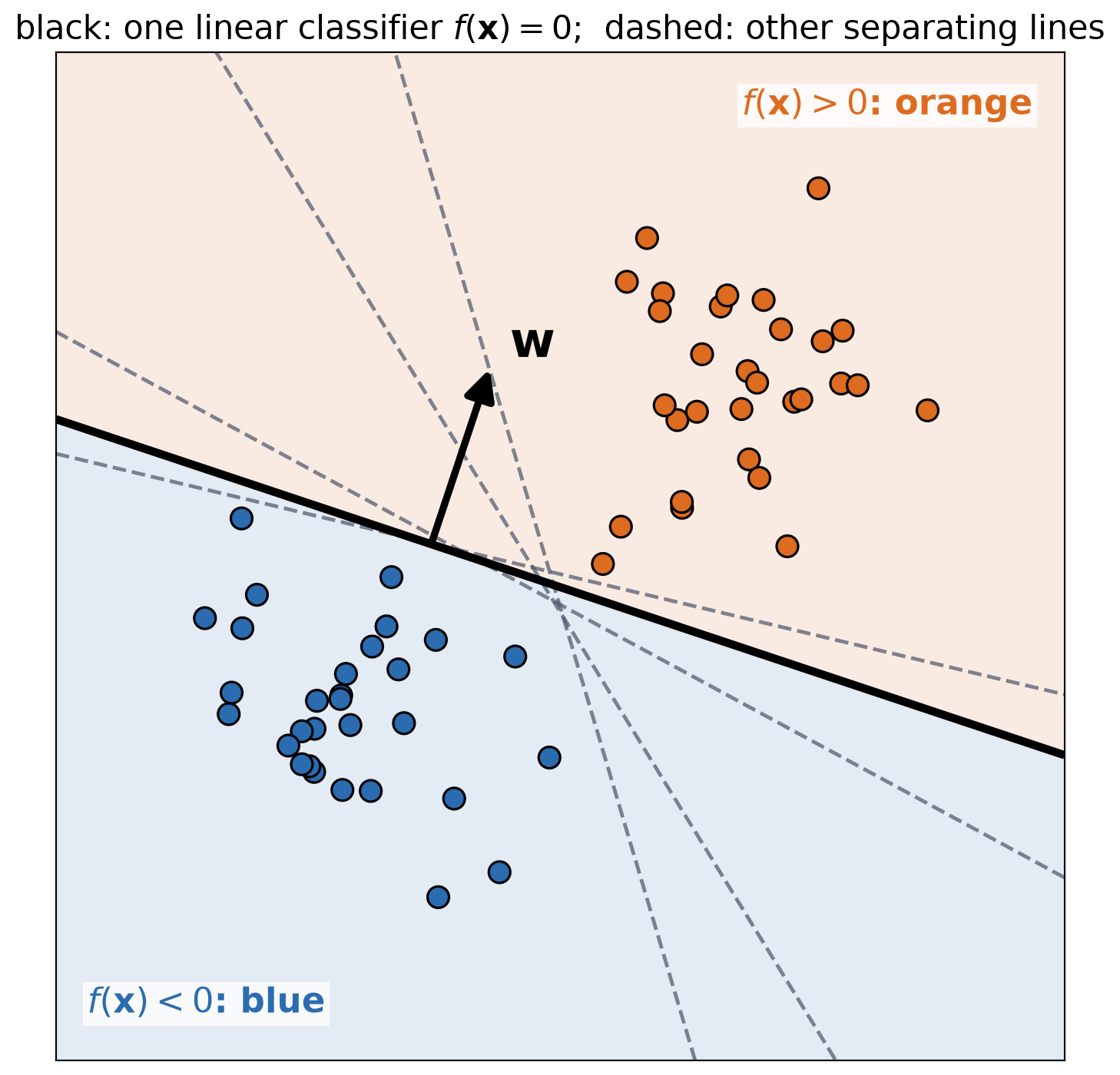
- A linear classifier scores an input with a weighted sum:
\[ \bbox[border: 2px solid #c53030; padding: 2px 6px]{f(\mathbf{x}) = \mathbf{w} \cdot \mathbf{x} + b}\;\;{\color{#c53030}{\begin{array}{l}\textbf{linear}\\ \textbf{classifier}\end{array}}} \]
\(\mathbf{x}\): input point coordinates.
\(\mathbf{w}\): weights; \(b\): bias. Both learned.
Predict orange if \(f(\mathbf{x}) > 0\), blue otherwise.
The decision boundary \(f(\mathbf{x}) = 0\) is a line (a “hyperplane” in more dimensions).
Many lines separate the training points (dashed). Which one is best?
Support Vector Machine (SVM)
- SVM (support vector machine): the linear classifier with the largest margin. A wide gap is safer for new points.
- Margin: the distance from the boundary to the closest training points.
- Support vectors: the points on or inside the margin. They alone fix the boundary; moving any other point changes nothing.

Soft Margin
- Overlapping classes: some points must be inside the margin or on the wrong side (soft margin).
- Hyperparameter \(C\): the penalty for those points.
- Small \(C\): wide margin, many points inside.
- Large \(C\): narrow margin, fewer points inside.
- Like \(k\), choose \(C\) on validation data.

Kernel SVM: Nonlinear Boundaries
- No line separates blue and orange points.
- Idea: map each point to a higher-dimensional space, where a plane separates them. Here: \((x_1,\, x_2) \mapsto (x_1,\, x_2,\, x_1^2 + x_2^2)\).
- A linear SVM in the new space is a nonlinear boundary in the original space (here: a circle).
- In practice, a kernel (e.g., RBF) builds the mapping inside the SVM; its hyperparameter \(\gamma\) sets how curvy the boundary can be.

Multi-Class SVM: One vs. Rest
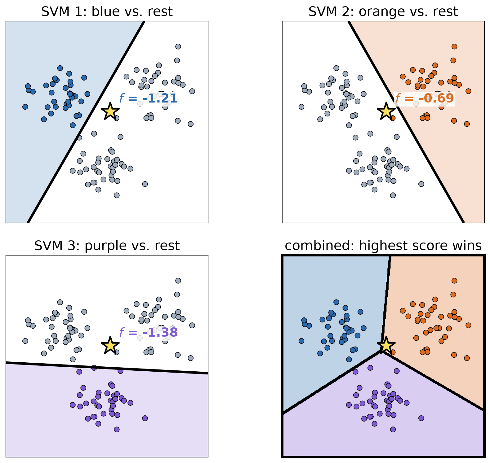
- Unfortunately, there is no definitive multi-class SVM. In practice, we combine multiple two-class SVMs.
One vs. Rest
- For each class \(c\): train a binary SVM, class \(c\) (+1) vs. all other classes (−1).
- New image: compute all class scores \(f_c(\mathbf{x})\).
- Predict the class with the highest score.
- 3 classes: 3 SVMs. 10 FashionMNIST classes: 10 binary SVMs.
- Star: \(f_{\text{blue}}\) = -1.21, \(f_{\text{orange}}\) = -0.69, \(f_{\text{purple}}\) = -1.38 \(\rightarrow\) predict orange.
Multi-Class SVM: One vs. One
One vs. One
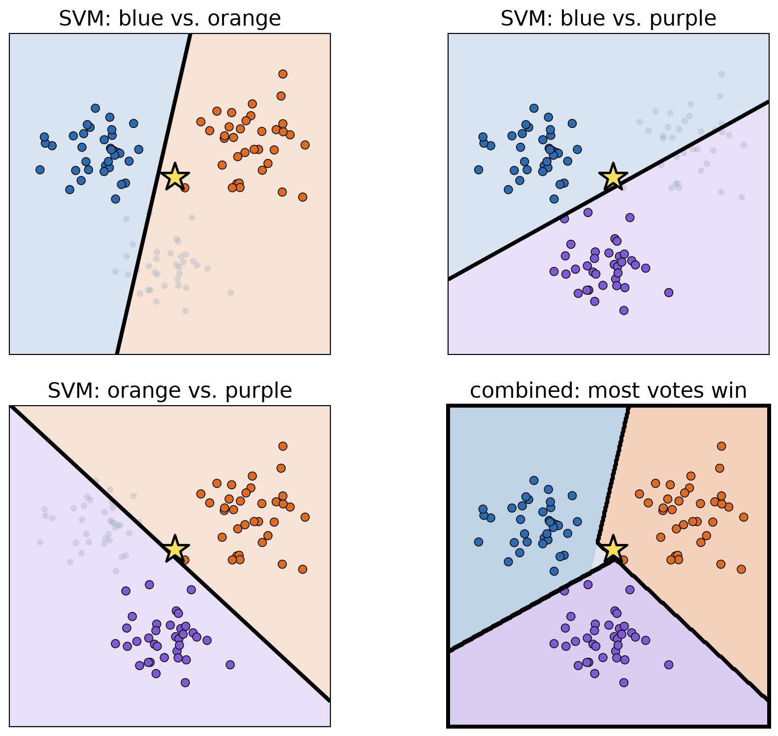
- For each pair of classes: train a binary SVM on the points of those two classes only.
- New image: each SVM votes for one of its two classes.
- Predict the class with the most votes.
- Star: votes 1 blue, 2 orange, 0 purple \(\rightarrow\) predict orange.
- OpenCV’s SVM handles multiple classes by itself, with one vs. one: one SVM per pair of classes, 45 SVMs for 10 classes, then a majority vote.
| One vs. rest | One vs. one | |
|---|---|---|
| SVMs for 3 classes | 3 | 3 |
| SVMs for 10 classes | 10 | 45 |
| Data per SVM | all images | images of 2 classes |
| Prediction | highest score | most votes |
Our FashionMNIST Benchmark
| Method | Input | Test accuracy | Training time | Time per image | Model size |
|---|---|---|---|---|---|
| KNN (\(k\) = 6) | 784 pixels | 85.0% | none | 1.4 ms | 157 MB |
| KNN (\(k\) = 6) | 50 PCA features | 85.6% | PCA only | 0.1 ms | 10 MB |
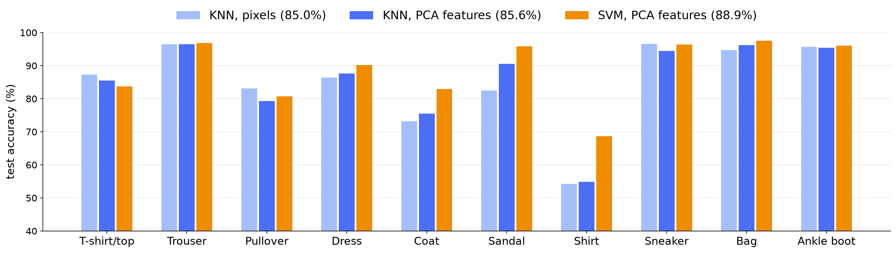
| SVM (RBF) | 50 PCA features | 88.9% | 16.5 s | 0.1 ms | 3.1 MB |
- SVM: best so far, +3.9 points over KNN on pixels.
- All three methods use pixel-based features. Neural networks learn their own features; we will compare them later.