Lecture 16 — Classical Object Detection

Lecture 16

Kaveh Fathian

Computer Science Department, Colorado School of Mines

Learning Objectives

By the end of this lecture, you should be able to:

  • Explain why raw pixels are poor features for pedestrians, and describe a window with HOG: gradient histograms in cells, normalized over blocks.
  • Classify a window with a linear SVM on its HOG vector.
  • Turn a classifier into a detector with sliding windows, an image pyramid, and non-maximum suppression (IoU).
  • Run the Dalal–Triggs pedestrian detector in OpenCV, step by step and with detectMultiScale.
  • Evaluate a detector with precision, recall, the precision–recall curve, and AP (and mAP).
  • Explain how Viola–Jones makes face detection fast: Haar features, the integral image, AdaBoost, and the attentional cascade.
  • Compute a rectangle sum and a Haar feature from the integral image, and run AdaBoost on a small example.
  • Detect faces with OpenCV’s CascadeClassifier, and recognize its limits.

Pedestrian Classification

Pedestrian Classification

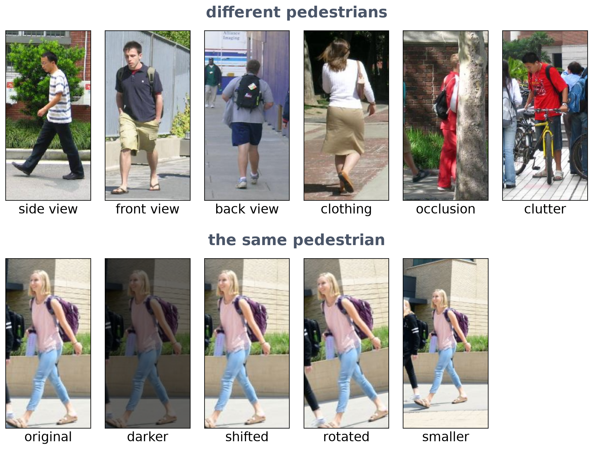
  • Pedestrian classification: is there a pedestrian in a 64 × 128 window or not?
  • Pedestrians look very different: pose, viewpoint, clothing, occlusion and background clutter.
  • The same pedestrian also changes with lighting, position, rotation and size in the window.
  • These changes alter the pixel values far more than they alter the person, so KNN or an SVM on raw pixels works poorly.
  • We need features that stay the same under these changes but still separate pedestrians from everything else.

Histogram of Oriented Gradients (HOG)

  • Idea: describe a window by its edge directions. The shape of a person is in the gradients, not in the pixel values.

HOG Descriptor

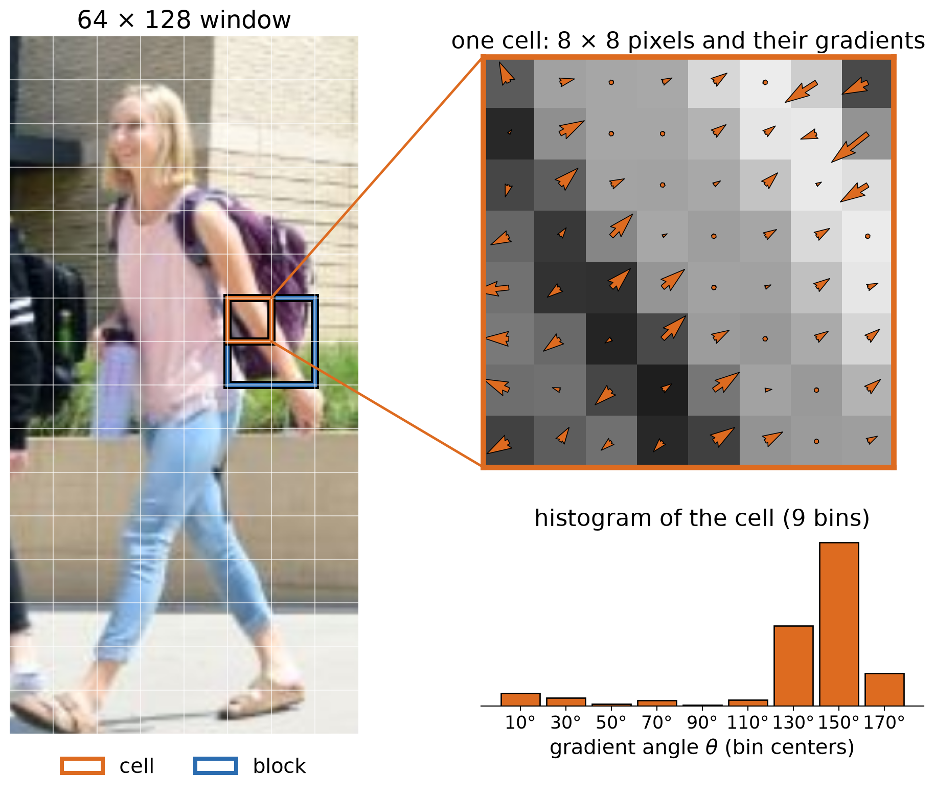
  1. Compute the gradient magnitude and angle at every pixel.
  2. Split the 64 × 128 window into 8 × 8-pixel cells.
  3. For each cell, a histogram of gradient angles: 9 bins over 0°–180°; each pixel adds its magnitude to the bin of its angle.
  4. Group 2 × 2 cells into a block and normalize it, so lighting changes cancel out.
  5. Concatenate all blocks into the HOG vector.
HOG Vector

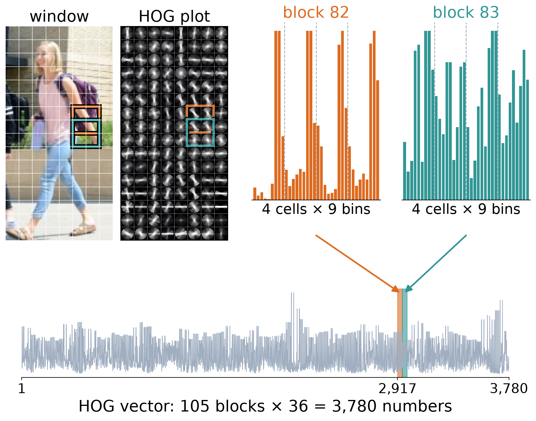
  • A window has 7 × 15 = 105 blocks of 2 × 2 cells. Neighboring blocks overlap by one cell.
  • Each block: its 4 cell histograms (36 numbers), normalized to unit length.
  • HOG vector: all normalized blocks, one after another: 105 × 36 = 3,780 numbers.
HOG + Linear SVM Classifier

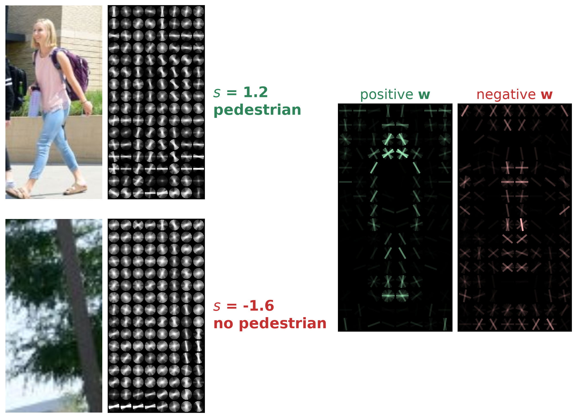
  • Classifier: a linear SVM on the HOG vector \(\mathbf{x}\) of the window:

\[ \bbox[border: 2px solid #c53030; padding: 2px 6px]{s = \mathbf{w}^\top \mathbf{x} + b}\;\;{\color{#c53030}{\textbf{pedestrian if } s > 0}} \]

  • Trained on HOG vectors of pedestrian windows (positive) and background windows (negative).
  • OpenCV includes a trained classifier: \(\mathbf{w}\) (3,780 weights) and \(b\).
  • Positive weights: where the SVM expects edges of a person. Negative weights: edges that suggest background.
From Classification to Detection

Pedestrian Detection

  • Pedestrian detection: draw a bounding box around every person in the image.
  • Idea: check every window. Slide the 64 × 128 window over the image, and classify each window.
  • Problems, and how to solve them:
    • Too many windows: move the window 8 pixels at a time (the stride). This image still has 7,524 windows.
    • People come in many sizes, but the window has one size: image pyramid.
    • A person gives positive scores in several overlapping windows: keep one box per person (non-maximum suppression).
Animation

Image Pyramids

  • People appear at many sizes, but the window has one size.
  • Image pyramid: shrink the image a little at a time (by a factor of 1.05), and slide the same window over every level.
  • Large people fit the window at small levels. Smaller people fit at larger levels.
  • A window found at scale \(s\) is a box \(1/s\) times larger in the original image.
  • This image: 34 levels and 63,958 windows in total.

Non-Maximum Suppression

  • Intersection over union (IoU): how much two boxes overlap.

\[ \bbox[border: 2px solid #c53030; padding: 2px 6px]{\text{IoU}(A, B) = \frac{\text{area}(A \cap B)}{\text{area}(A \cup B)}}\;\;{\color{#c53030}{\textbf{IoU}}} \]

Non-Maximum Suppression (NMS)

  1. Drop all windows with a score below a threshold (e.g., \(s < 0.5\)).
  2. Pick the highest-scoring remaining window and add it to the detections.
  3. Delete all remaining windows that overlap it with IoU > 0.3 (they show the same person).
  4. Repeat steps 2–3 until no windows remain.

Dalal–Triggs Pedestrian Detector

Dalal–Triggs Detector

  1. Build an image pyramid.
  2. Slide a 64 × 128 window over every level.
  3. Compute the window’s HOG vector \(\mathbf{x}\).
  4. Linear SVM score: \(s = \mathbf{w}^\top \mathbf{x} + b\).
  5. Keep windows with \(s\) above a threshold, and apply NMS.
  • The same classifier, applied to every window at every scale, turns classification into detection.

Dalal–Triggs Detector in Code

  • HOGDescriptor(): the Dalal–Triggs settings (64 × 128 window, 8 × 8 cells, 2 × 2-cell blocks, 9 bins).
  • getDefaultPeopleDetector(): the trained \(\mathbf{w}\) and \(b\).
  • groupThreshold=0: all windows with \(s > 0\), at every scale. NMSBoxes then applies NMS.
  • Full detector: detectMultiScale alone runs every step, but merges overlapping windows with its own grouping instead of NMS.
hog = cv2.HOGDescriptor()
svm = cv2.HOGDescriptor_getDefaultPeopleDetector()
w, b = svm[:-1], svm[-1]             # 3,780 weights, bias

# Classify one 64 x 128 window
window = cv2.resize(image[y0:y1, x0:x1], (64, 128))
x = hog.compute(window)              # HOG vector
s = w @ x + b                        # pedestrian if s > 0

# Detect: all windows with s > 0, then NMS
hog.setSVMDetector(svm)
boxes, scores = hog.detectMultiScale(
    image, winStride=(8, 8), scale=1.05, groupThreshold=0)
keep = cv2.dnn.NMSBoxes(boxes, scores, 0.5, 0.3)
# Full detector in one call
hog = cv2.HOGDescriptor()
hog.setSVMDetector(
    cv2.HOGDescriptor_getDefaultPeopleDetector())
boxes, scores = hog.detectMultiScale(
    image, winStride=(8, 8), scale=1.05)

Dalal–Triggs Detector: Full Code

import cv2
import numpy as np
import matplotlib.pyplot as plt

image = cv2.imread("assets/16_classical_detection/people.jpg")

# 1. HOG with the Dalal–Triggs settings, and OpenCV's trained linear SVM.
hog = cv2.HOGDescriptor()
print("HOG vector length:", hog.getDescriptorSize())          # 3,780
svm = cv2.HOGDescriptor_getDefaultPeopleDetector()            # 3,780 weights w, then the bias b
w, b = svm[:-1], svm[-1]
hog.setSVMDetector(svm)

# 2. Image pyramid (scale 1.05), sliding windows (stride 8) and SVM scores.
#    groupThreshold=0 returns every window with s > 0, without merging.
boxes, scores = hog.detectMultiScale(image, winStride=(8, 8), scale=1.05, groupThreshold=0)
scores = scores.ravel()
print("windows with s > 0:", len(boxes))

# 3. Non-maximum suppression: drop scores below 0.5, then remove boxes with IoU > 0.3
#    with a higher-scoring box.
keep = np.ravel(cv2.dnn.NMSBoxes(boxes.tolist(), scores.tolist(), 0.5, 0.3))
boxes, scores = boxes[keep], scores[keep]
print("detections after NMS:", len(boxes))

# 4. Classify one window by hand: s = w . x + b for the window of the best detection.
x0, y0, bw, bh = boxes[np.argmax(scores)]
window = cv2.resize(image[y0:y0 + bh, x0:x0 + bw], (64, 128), interpolation=cv2.INTER_AREA)
x = hog.compute(window)                                       # HOG vector of the window
print(f"score of the window: {w @ x + b:.1f}")

# 5. Draw the detections and their scores.
out = cv2.cvtColor(image, cv2.COLOR_BGR2RGB)
for (bx, by, bw, bh), s in zip(boxes, scores):
    cv2.rectangle(out, (bx, by), (bx + bw, by + bh), (0, 200, 0), 2)
    cv2.putText(out, f"{s:.1f}", (bx + 3, by + 18), cv2.FONT_HERSHEY_SIMPLEX, .6, (0, 200, 0), 2)
plt.imshow(out)
plt.axis("off")
plt.show()

Evaluating Detectors

Precision and Recall

  • Compare the detections with the ground-truth boxes (labeled by hand).
  • True positive (TP): a detection with IoU ≥ 0.5 with a ground-truth box. Each ground-truth box can be matched only once.
  • False positive (FP): any other detection.
  • False negative (FN): a person with no matching detection.

\[ \bbox[border: 2px solid #c53030; padding: 2px 6px]{\text{precision} = \frac{TP}{TP + FP}}\;\;{\color{#c53030}{\begin{array}{l}\textbf{how many}\\ \textbf{detections}\\ \textbf{are correct}\end{array}}} \]

\[ \bbox[border: 2px solid #c53030; padding: 2px 6px]{\text{recall} = \frac{TP}{TP + FN}}\;\;{\color{#c53030}{\begin{array}{l}\textbf{how many}\\ \textbf{people}\\ \textbf{are found}\end{array}}} \]

TP = 1, FP = 1, FN = 1: precision = 0.50, recall = 0.50

Precision–Recall Curve

  • Keep only the detections whose score \(s\) is above a threshold.
  • High threshold: few detections, mostly correct: high precision, low recall.
  • Low threshold: more people found, but more false positives: higher recall, lower precision.
  • Precision–recall curve: precision and recall as the threshold goes down (also below 0), until recall stops increasing.
Animation

Average Precision (AP)

  • One number for the whole curve: the area under the precision–recall curve.

\[ \bbox[border: 2px solid #c53030; padding: 2px 6px]{\text{AP} = \text{area under the curve}}\;\;{\color{#c53030}{\begin{array}{l}\textbf{higher}\\ \textbf{is better}\end{array}}} \]

  • Dalal–Triggs on all 170 Penn-Fudan images: AP = 0.34. Even with every window, recall stops at 0.72.
  • mAP (mean average precision): with several object classes, compute the AP of each class and take the mean.

Viola–Jones Face Detection

Viola–Jones Face Detector

  • Face detection: draw a box around every face.
  • Same approach as for pedestrians: classify every window (24 × 24 pixels) at every scale of an image pyramid.
  • Faces are rare and windows are many, so each window must be classified very fast.
  • Four ideas make it fast:
    1. Haar features
    2. Integral image
    3. Boosting
    4. Attentional cascade.

Haar Features

  • A Haar feature is a pattern of adjacent white and black rectangles.
  • Its value: the sum of the pixels under white minus the sum of the pixels under black, which measures a brightness difference.
  • Every position and size of the five types fits in a 24 × 24 window: 162,336 features.
  • Viola–Jones uses only these five types (upright rectangles).

Integral Image

  • Integral image: each pixel holds the sum of all pixels above and to the left of it (including itself).

\[ \bbox[border: 2px solid #c53030; padding: 2px 6px]{\text{sum} = D - B - C + A}\;\;{\color{#c53030}{\textbf{4 lookups}}} \]

  • With the integral image, any rectangle sum takes 4 lookups, and any Haar feature only a few (6–9), whatever its size.
  • Bottom: a two-rectangle feature. Its rectangles share 2 corners: 6 lookups.
Animation

AdaBoost

  • Decision stump \(h\): threshold one feature, e.g., \(h(\mathbf{x}) = +1\) if \(x_1 > 0.4\), else \(-1\). In 2D: a vertical or horizontal line.

AdaBoost

  1. Same weight for all \(n\) points: \(w_i = 1/n\).
  2. Pick the stump \(h_t\) with the smallest weighted error \(\varepsilon_t\) (total weight of its wrong points).
  3. Its vote: \(\alpha_t = \frac{1}{2}\ln\frac{1 - \varepsilon_t}{\varepsilon_t}\).
  4. Wrong points: weight \(\times\, e^{\alpha_t}\). Correct points: \(\times\, e^{-\alpha_t}\). Normalize.
  5. Repeat 2–4. Final: \(H(\mathbf{x}) = \text{sign}\big(\sum_t \alpha_t h_t(\mathbf{x})\big)\).
  • Stop: after a set number of rounds, or once accurate enough (here: no mistakes after 3 rounds).
Animation

Boosting with Haar Features

  • Weak classifier: a decision stump on one Haar feature value.
  • Training (once): each boosting round adds the best of the 162,336 features. A stage stops when it meets its target. Viola–Jones in OpenCV keeps 2,913 features in total.
  • Detection: only these features are computed.
  • The first two features of OpenCV’s face cascade:
    • eyes darker than the forehead and cheeks;
    • bridge of the nose brighter than the eyes.

Attentional Cascade

  • Most windows are clearly not faces: reject them early, with only a few features.
  • Cascade: a chain of boosted classifiers that grow stronger. A 24 × 24-pixel window is a face only if it passes every stage.
  • Viola–Jones in OpenCV: 25 stages; stage 1 has 9 features, stage 25 has 200.
  • Example: each stage keeps 99.5% of faces and passes 50% of non-faces:
    • Faces kept: \(0.995^{25} \approx 88\%\)
    • Non-faces passed: \(0.5^{25} \approx 3 \times 10^{-8}\)
Animation

Viola–Jones in Code

  • CascadeClassifier(file): loads a trained cascade.
  • detectMultiScale(gray, scaleFactor, minNeighbors): pyramid, sliding window and cascade.
  • minNeighbors: keep only places with at least this many overlapping detections, and merge them into one box (instead of NMS).
  • Finds only frontal, upright faces.
  • OpenCV 5 doesn’t include the trained cascades: download them from OpenCV’s GitHub.
cascade = cv2.CascadeClassifier(
    "haarcascade_frontalface_default.xml")
gray = cv2.cvtColor(image, cv2.COLOR_BGR2GRAY)
faces = cascade.detectMultiScale(
    gray, scaleFactor=1.1, minNeighbors=5)  # (x, y, w, h)

Viola–Jones: Full Code

import time
import xml.etree.ElementTree as ET

import cv2
import matplotlib.pyplot as plt

# OpenCV 5 doesn't include the trained cascades. Download haarcascade_frontalface_default.xml from
# https://github.com/opencv/opencv/tree/4.x/data/haarcascades
folder = "assets/16_classical_detection/"
cascade_file = folder + "haarcascade_frontalface_default.xml"
image = cv2.imread(folder + "faces.jpg")

# 1. The trained cascade: stages and features per stage (from the .xml file).
stages = ET.parse(cascade_file).getroot()[0].find("stages")
sizes = [int(s.find("maxWeakCount").text) for s in stages]
print(f"{len(sizes)} stages, {sum(sizes)} features; first stages: {sizes[:3]}")

# 2. Detect: image pyramid (scale 1.1), sliding 24 x 24 window, cascade, and merging of
#    overlapping detections (at least 5 neighbors).
cascade = cv2.CascadeClassifier(cascade_file)
gray = cv2.cvtColor(image, cv2.COLOR_BGR2GRAY)
t0 = time.perf_counter()
faces = cascade.detectMultiScale(gray, scaleFactor=1.1, minNeighbors=5)
print(f"{len(faces)} faces in {time.perf_counter() - t0:.1f} s")

# 3. Draw the detections.
out = cv2.cvtColor(image, cv2.COLOR_BGR2RGB)
for x, y, w, h in faces:
    cv2.rectangle(out, (x, y), (x + w, y + h), (0, 200, 0), 2)
plt.imshow(out)
plt.axis("off")
plt.show()

Key Takeaways

  • HOG describes a window by its edge directions: gradient histograms in 8 × 8 cells, normalized over 2 × 2-cell blocks. A linear SVM scores it: \(s = \mathbf{w}^\top \mathbf{x} + b\).
  • Classification → detection: classify every window at every level of an image pyramid, then NMS keeps one box per object.
  • A detection is a true positive if its IoU with a ground-truth box is ≥ 0.5. Lowering the threshold trades precision for recall. AP is the area under the precision–recall curve; mAP is its mean over classes.
  • Viola–Jones makes each window cheap: Haar features are brightness differences of rectangles, computed in a few lookups with the integral image (\(D - B - C + A\)).
  • AdaBoost combines weak stumps: each round picks the stump with the lowest weighted error, gives it a vote \(\alpha_t\), and increases the weight of its mistakes.
  • The attentional cascade rejects most windows in the first stages, with only a few features. Only face-like windows reach the later stages.
  • Both detectors use hand-designed features; neural networks learn the features from data.